Introduction
Screencast video [⯈]
Module overview
This module will cover one of the most fundamental aspects in signal processing, namely the principle behind converting a continuous-time signal into a discrete-time signal in order to process it with the help of computers.
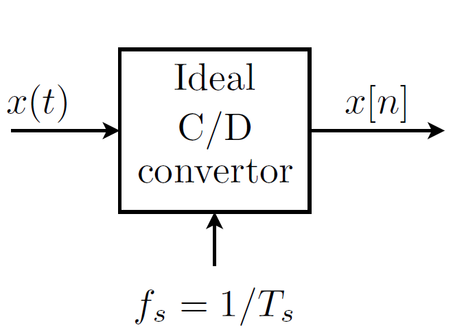
- Sampling of sinusoidal signals - First the concept of sampling is discussed, which represents the conversion from the continuous-time to discrete-time domain. The frequency of the sampled signal is better to be described by a relative frequency, because of the effect of the sampling process. Through the sampling there can also be a loss of spectral information, known as aliasing. This is caused by the uniqueness issue.
- Reconstruction of sinusoidal signals [⯈] - Similarly to the sampling, the signal can also be converted back from the discrete-time domain to the continuous-time domain. In order to prevent aliasing the sampling theorem has to be satisfied.
- Examples [⯈] - In order to get the reader more acquainted with the sampling procedure, this section includes a screencast video with several examples.
Exercises
In this section several exercises are available, including their answers. The exercises marked in blue are explained by means of more extensive pencast videos.
Video quiz
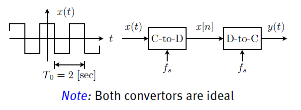
case 1: $f_s = f_{s1} \rightarrow x_1[n]=\cos(\theta_1 n)$
case 2: $f_s = 1/3\cdot f_{s1} \rightarrow x_2[n]=\cos(\theta_2n)$
In the equation $\theta_2= \alpha\cdot \theta_1$, what is the value of $\alpha$?
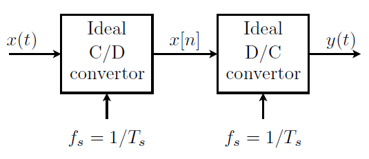
What is the minimal sampling rate $f_s$ to obtain no aliasing, thus $y(t)=x(t)$.
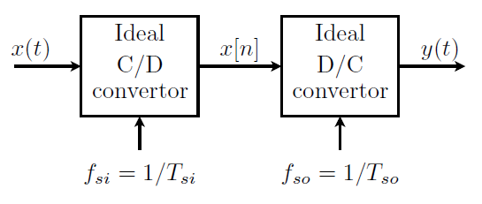
$f_{si} = 500$ [samples/sec]
$f_{so} = 400$ [samples/sec]
$x(t) = \cos(2\pi\cdot100t)$ and $y(t) = \cos(2\pi\cdot f_y t)$
What is the value of $f_y$?
Exercise bundle
Answers
Download the answers here.
Pencast videos [⯈]
The above video player contains a playlist of all pencast videos which can be expanded by clicking the playlist icon in the upper-right corner.
MATLAB lab
Accompanied to this modules are some exercises in MATLAB, which will test your knowledge of the module and will help improve your MATLAB skills.
Lab assignment
MATLAB demo [⯈]
Summary
$$ \text{Relation absolute- and relative- frequency:} \qquad \boxed{\theta = \omega \cdot T_s= 2 \pi \frac{f}{f_s}} $$
| Frequency | Symbol | Unit |
|---|---|---|
| Absolute frequency | $f$ | [Hz] |
| Absolute radial frequency | $\omega$ | [rad/sec] |
| Relative frequency | $\theta$ | [-] |
| Frequency | Symbol | Fundamental Interval |
|---|---|---|
| Relative frequency | $\theta$ | $-\pi < \theta \leq \pi$ |
| Absolute frequency | $f$ | $-\frac{f_s}{2} < f \leq \frac{f_s}{2}$ |
| Absolute radial frequency | $\omega$ | $-\pi f_s < \omega \leq \pi f_s$ |