Spectrum of sinusoidal signals

Introduction

Many practical signals can be described as a set of sinusoidal signals. In this module we will first show how such a set can be rewritten as a set of weighted phasor components. From this description it follows that these weights represent the spectral information of the signal.

Screencast video [⯈]

Module overview

This module covers the following topics:

1. Real signal as sum of phasors - This section will show that every real signal can be decomposed in the sum of complex phasors.
2. Spectral plot - Since a signal can be decomposed in a sum of phasors with different frequencies, it is also possible to represent this graphically in a spectral plot.
3. Product versus sum of sinusoids - Summing sinusoidal signals will simply results in a spectrum composed out of the combined original spectral components. However, the multiplication of two sinusoidal signals (better known as modulation) will have different consequences for the spectrum.
4. Special cases [⯈] - This module will end with a brief section in which several special spectra are discussed.

Exercises

In this module several exercises are available, including their answers. The exercises marked in blue are explained by means of more extensive pencast videos. These exercises also include topics relating to the Fourier series.

Video quiz

Test your knowledge (click to expand)

Question 1

Which spectral plot corresponds to the complex signal $z(t) = 2e^{-j(2\pi t - \frac{\pi}{6})}$?

None of the answers is correct.

Question 2

Which spectral plot corresponds to the signal $x(t) = 2 \cos(2\pi\cdot 100t - \frac{\pi}{3})$?

None of the answers is correct.

Question 3

Which signal corresponds to the following spectral plot?

$x(t) = 2\sin(20\pi t - \frac{\pi}{3})$
$x(t) = \cos(20\pi t - \frac{\pi}{3})$
$x(t) = 2\sin(20\pi t + \frac{\pi}{3})$
$x(t) = \cos(20\pi t + \frac{\pi}{3})$
None of the answers is correct.

Question 4

Which signal corresponds to the following spectral plot?

$x(t) = 2\sin(2\pi t) + 4\cos(4\pi t +\frac{\pi}{4})$
$x(t) = 2\cos(2\pi t) + 4\cos(4\pi t -\frac{\pi}{4})$
$x(t) = 2\cos(2\pi t) + 4\cos(4\pi t +\frac{\pi}{4})$
$x(t) = 2\sin(2\pi t) + 4\cos(4\pi t -\frac{\pi}{4})$

Question 5

Consider the spectral plot of an amplitude modulated signal depicted in the figure below. The signal is the porduct of the carrier signal $g(t)$ multiplied with the message signal $s(t)$. The signal $s(t)$ can be written as $s(t) = A_0 + A_1\cos(2\pi f_1 t + \Phi_1)$. Compute the parameters $A_0$, $A_1$, $f_c$, $f_1$ and $\Phi_1$.

$A_0 = 1$, $A_1= \frac{1}{4}$, $f_c= 5000$ Hz, $f_1 = 750$ Hz and $\Phi_1=\frac{\pi}{4}$
$A_0 = 2$, $A_1= 1$, $f_c= 5000$ Hz, $f_1 = 750$ Hz and $\Phi_1=-\frac{\pi}{4}$
$A_0 = 2$, $A_1= 1$, $f_c= 750$ Hz, $f_1 = 5000$ Hz and $\Phi_1=\frac{\pi}{4}$
None of the answers is correct.

Exercise bundle

Answers

Download the answers here.

Pencast videos [⯈]

The above video player contains a playlist of all pencast videos which can be expanded by clicking the playlist icon in the upper-right corner.

Summary

• Sum of DC and $N$ sinusoids written as sum of phasors: $$ \begin{split} x(t) &= A_0 + \sum_{k=1}^{N} A_k\cos \left( 2\pi f_k t+ \phi_k \right),\newline &= X_0 + \sum_{k=1}^N \bigg\{ \frac{X_k}{2}e^{j2\pi f_k t} + \frac{X_k^\ast}{2}e^{-j2\pi f_k t} \bigg\}, \end{split} $$

  where $X_0 = A_0$ and $X_k = A_ke^{j\phi_k}$.

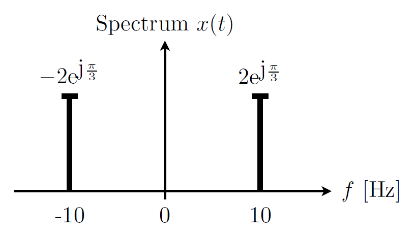
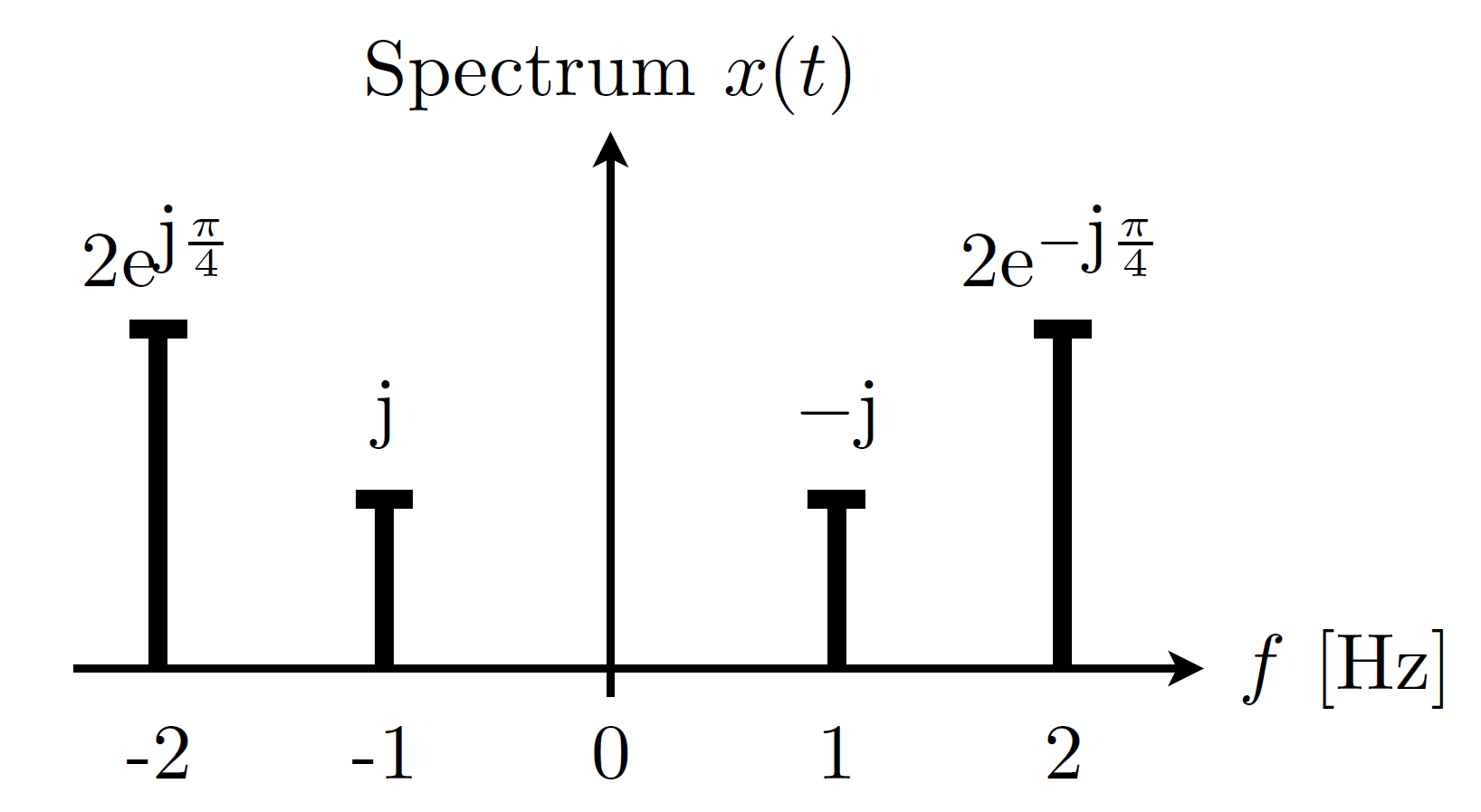
  For real signals the values of the complex weights of the phasors with negative frequencies are the complex conjugated versions of the complex weights of the phasors with positive frequencies.
• By ordering the frequencies from low to high we can represent the phasor description in a frequency spectrum plot. In such a plot we denote the frequencies on the horizontal axis. The frequency on this axis can either be denoted by the values of $f_k$ in [Hz] or by the values of $\omega_k = 2\pi f_k$ in [rad/sec]. For each of these frequencies $f_k$ we plot a bar, denoting the complex weights $\frac{X_k}{2}$. These complex weights are related to the magnitude and phase of the original sinusoidal signal.
  It is easiest to denote the complex numbers of the bars in the spectral plot in Polar notation.
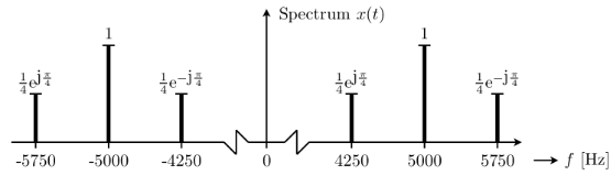
• A product of sinusoids is related to a sum of sinusoids:
  We can write the product of two sinusoidal signals with frequencies $f_c$ and $f_\Delta$ as the sum of two sinusoidal signals with frequencies $f_c-f_\Delta$ and $f_c+f_\Delta$
• An Amplitude Modulated (AM) signal has the following property:
  When a message signal $m(t)$ is modulated by a carrier signal $c(t)$ with frequency $f_c$, the whole spectral content of the message is moved to both the positive and negative frequency component of the carrier signal.