3.3 Parametric spectral estimation

Non-parametric spectral estimation methods are based on two major assumptions. First of all, by the calculation of the Fourier transform it is assumed that our finite signal is periodic. The period in this case is fixed by the length of the signal $N$. Because the signal is unknown, it is highly unlikely that this assumption is actually valid. Secondly, the estimated auto-correlation function of the finite signal is zero for absolute lags larger than the signal length. Because the auto-correlation has now also a finite window, the indirect method cannot calculate the exact power spectral density, limiting the resolution of the estimate.

It would be nice to extrapolate the auto-correlation function for larger lags, because this would increase the resolution of the estimated power spectral density. With extrapolation we are referring to the process where additional values are estimated or predicted based on the already available information. In other words, the auto-correlation function can be extended or extrapolated by finding a pattern in the available auto-correlation function and by filling the unknown values with the expected values from this pattern.

This pattern or signal model requires us to have some prior information about the signal generating process, otherwise it is impossible to determine an accurate signal model that would correspond to the obtained auto-correlation function. After the signal model has been identified, it needs to be fitted to the available auto-correlation function. This means that the unknown parameters of the signal model are estimated according to the available auto-correlation function, and once the parameters are estimated, the signal model can be used to estimate the entire auto-correlation function.

This approach is very different from the non-parametric methods and it is usually referred to as parametric method, by which parameters of a signal model are estimated such that signal and auto-correlation function can be described by such a model. The parametric approach roughly consists of three steps. First, a signal model needs to be defined. This step is usually the hardest since it would ideally require prior knowledge on the random process. If this knowledge is not available, then several models can be fitted to the data after which the most optimal is chosen. The definition of optimal depends on the evaluation criterion. Once the model is defined, the second step is to estimate the parameters of the model based on the available date (finite-length signal or autocorrelation function). Finally, the last step is to obtain the power spectral density using the signal model.

Rational signal models

The first step in estimating the power spectral density is finding a signal model. How do we define such a signal model? One way is to use spectral factorization, i.e., modeling the signal as obtained by filtering a white Gaussian process $i[n]$ by a linear time-invariant (LTI) filter. A white Gaussian process has the characteristic that the power spectral density is constant. If we transform this constant spectrum by applying filters (low-pass, high-pass etc.), it is possible to shape the power spectral density in a controlled way. In other words a constant spectrum can be filtered such that the resulting spectrum provides us with a good estimate of the power spectral density of the observed random signal. Of course, we cannot directly assess the accuracy of the resulting spectrum since this is unknown, but we can compare the estimated with the determined auto-correlation functions. Although in principle there is an infinite number of possibilities for the filter, we typically restrict the choice to finite impulse response (FIR) and infinite impulse response (IIR) filters. This is equivalent to modeling the random signal as an ARMA process.

Screencast video [⯈]

Stochastic signal modeling and auto-regressive moving-average (ARMA) processes were discussed in detail in the section Rational signal models. Here we briefly review some important concepts, which are useful for the purpose of parametric spectral estimation.

AR($p$) spectral estimation

AR($p$) process

An auto-regressive process of order $p$ is defined by the following difference equation \begin{equation} x[n] = i[n] - a_1 x[n-1] - a_2 x[n-2] - \ldots - a_p x[n-p], \end{equation} where $i[n]$ is the input white noise and $a_i$ are the filter coefficients.

The transfer function can be found as \begin{equation} \begin{split} H(z) = \frac{1}{1+\sum_{p=1}^{P} a_p z^{-p}} = \frac{1}{A(z)}. \end{split} \end{equation} The auto-correlation function is given by \begin{equation} \sigma_i^2\delta[l] = \sum_{k=0}^p a_k r_x[l-k], \end{equation} or equivalently \begin{equation} r[l] = - \sum_{k=1}^p a_k r_x[|l|-k]. \end{equation}

When a windowed signal is observed and the auto-correlation function is estimated as $\hat{r}_x[l]$, the Yule-Walker equations can be used to estimate parameters $\hat{a}_1$,…, $\hat{a}_p$ and $\hat{\sigma}_i^2$. Since there are $p+1$ unknowns, we require $p+1$ equations to solve the Yule-walker equations, which is equivalent to using $p+1$ estimated correlation lags. The Yule-Walker equations for an AR process are linear, and thus can be written in a matrix form as

\begin{equation} \begin{bmatrix} \hat{r}_x[0] & \hat{r}_x[1] & \hat{r}_x[2] & \cdots & \hat{r}_x[p] \newline \hat{r}_x[1] & \hat{r}_x[0] & \hat{r}_x[1] & \cdots & \hat{r}_x[p-1] \newline \hat{r}_x[2] & \hat{r}_x[1] & \hat{r}_x[0] & \cdots & \hat{r}_x[p-2] \newline \vdots & \vdots & \vdots & \ddots & \vdots \newline \hat{r}_x[p] & \hat{r}_x[p-1] & \hat{r}_x[p-2]& \vdots & \hat{r}_x[0] \end{bmatrix} \begin{bmatrix} 1 \newline \hat{a}_1 \newline \hat{a}_2 \newline \vdots \newline \hat{a}_p \end{bmatrix} = \begin{bmatrix} \hat{\sigma}_i^2 \newline 0 \newline 0 \newline \vdots \newline 0 \end{bmatrix} \end{equation} Here we assume the signal $x[n]$ to be real, and thus a symmetric auto-correlation function of the form $\hat{r}_x[l] = \hat{r}_x[-l]$. Solving this system of equations, the unknown filter coefficient $\hat{a}_1, …, \hat{a}_p$, and unknown variance of the input noise in the model, $\hat{\sigma}_i^2$, can be estimated by least-square linear estimation. Note that the autocorrelation matrix as Toeplitz structure, which is a matrix with constant diagonals.

Finally, the power spectral density of an AR process is given by

\begin{equation}\label{eq:psd_AR} P_X(e^{j\theta}) = \frac{\sigma_i^2}{|1+a_1 e^{-j\theta} + a_2 e^{-j2\theta} + \ldots + a_p e^{-jp\theta}|^2}. \end{equation}

Estimation of an AR(p) spectrum

In order to estimate the spectrum of an AR(p) process the first step is to write down the Yule-Walker equations for a certain model order $p$. This model order can be freely chosen, but its performance can be measured using the metrics that will be discussed later on. To obtain the Yule-Walker equations, first the auto-correlation function of the signal should be estimated for lags $|l| \leq p$. From this equations, the AR coefficients $\hat{a}_i$ and the innovation variance $\hat{\sigma}^2_i$ can then be calculated. With these parameters the analytical AR power spectral density can be estimated using (\ref{eq:psd_AR}). For practical implementations, however, the power spectral density is often calculated using the DFT, zero-padded to length $L$, through \begin{equation} \hat{P}[k] = \frac{\hat{\sigma}_i^2}{\left| \sum_{i=0}^p \hat{a}_ie^{-jik\frac{2\pi}{L}}\right|^2}. \end{equation}

Calculation of AR parameters via 1-step linear predictor

An alternative way to calculate the AR model parameters $a_1, a_2, …, a_p$ and $\sigma_i^2$ is to use a 1-step linear predictor. This can be implemented as FIR Wiener filter. As shown in Fig. 1, the general goal of Wiener filters is to filter a signal $x[n]$ such to minimize the error between the filtered signal $\hat{x}[n]$ and a desired signal $d[n]$ according to the minimum mean square error (MMSE) criterion.

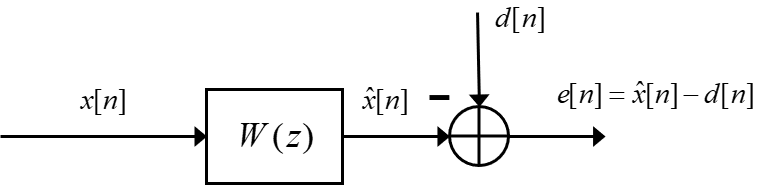
The general FIR solution for this Wiener filter is found by finding the set of parameters that minimizes a cost function defined as: \begin{equation} J=\mathrm{E}\left[e^2[n]\right] =\mathrm{E}\left[(d[n] - \hat{x}[n])^2\right] =\mathrm{E}\left[d[n]^2\right] - \bf{w}^T\bf{r_{dx}}-\bf{r_{dx}}^T\bf{w} + \bf{w}^T\bf{R_x}\bf{w} \end{equation}

where $\bf{w}$ is the vector composed of the filter coefficients, $\bf{r_{dx}}$ is the cross correlation between the desired and observed signals, and $\bf{R_x}$ is the autocorrelation matrix of the observed signal. The optimal filter coefficients $\bf{w_{opt}}$ can be found as the solution to the following minimization problem: $$ \mathbf{w_{opt}} = \arg\min_{w} (J) =\arg\min_{w} (\mathrm{E}\left[e^2[n]\right]), $$

By setting the derivative of $J$ equal to zero, the so-called normal equations are found as \begin{equation}\label{eq:normaleq} \frac{dJ}{dw}=2(\bf{r_{dx}}-\bf{R_x}\bf{w}) = 0 \hspace{1cm} \Longrightarrow \hspace{1cm} \bf{R_x}\bf{w} = \bf{r_{dx}}. \end{equation}

From (\ref{eq:normaleq}) the solution of the FIR Wiener filter is found as \begin{equation}\label{eq:wopt} \mathbf{w_{opt}} = \bf{R_x}^{-1}\bf{r_{dx}}. \end{equation} Moreover, the filter error can be calculated as \begin{equation}\label{eq:Jfir} J_{\text{FIR}} = r_d[0] - \sum_{i=0}^{N-1}w_{opt}[i] r_{dx}[i] = r_d[0] - \mathbf{w_{opt}}^T \mathbf{r_{dx}}. \end{equation}

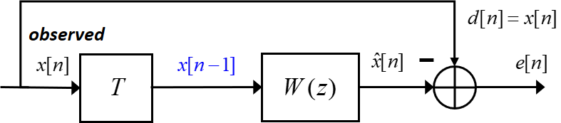
The goal of a 1-step linear predictor is to estimate the next value of the signal based on a linear combination of the past values of the signal. In this case, as schematically shown in Fig. 2, the input to the filter is a delayed version of the observed signal and the desired signal is the observed signal itself. For a 1-step linear predictor, the delay is $T=1$.

The solution of this filter is found by using (\ref{eq:wopt}) and substituting for $\bf{R_x}$ a matrix obtained using autocorrelation lags from $0$ up to $N-2$, where $N$ is the signal length; this means using the original signal as the desired signal. While for the cross-covariance $\bf{r_{dx}}$ we use the autocorrelation of $x[n]$, since in this case the input to the filter is a shifted version of the desired signal, and both are the observed signal $x[n]$; thus $\bf{r_{dx}} = \bf{r_{x}}$ using lags from $1$ up to $N-1$. In formulas this can be described as

\begin{equation} \mathbf{R_x}= \text{Toeplitz} [r_x[0], r_x[1], …, r_x[N-2]] \end{equation}

\begin{equation} \mathbf{r_{x}} = [r[1], r[2], …, r[n-1]]^T. \end{equation}

For an AR model, our signal is given by the sum of an unpredictable part and a predictable part composed of filtered past signal samples, that is

$x[n]=i[n]+\hat{x}[n]=i[n]-a_1x[n-1]+…-a_px[n-p]$.

Then, since the filter error is given by $x[n]-\hat{x}[n]=i[n]$, we are basically left with white noise. As a result the expected squared error is $E\{(x-x[n])^2\}=\sigma_i^2$.

When we want to use this filter to estimate the AR parameters $a_1, a_2, …, a_p$ and $\sigma_i^2$, we should bare in mind that the observed signal is actually modeled as the output of an LTI with $p$ poles and no zeros driven by white noise, as shown in Fig. 3.

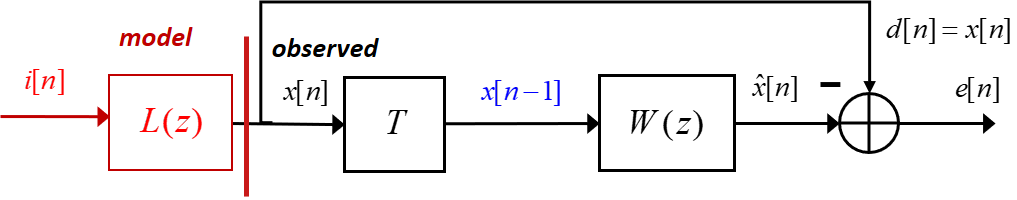
This means that the optimal filter $W(z)$ is actually the inverse of $L(z)$. In fact, $W(z)$ can be interpreted as a whitening filter that takes as input a random signal constituted by a predictable part and an unpredictable part and outputs white noise, that is the unpredictable part. Because of this, to obtain our AR model parameters, we need to invert the sign of the filter coefficients, while the input noise variance can be simply found by applying the formula for the filter error, as given below

\begin{equation} \mathbf{w_{opt}} = [w_1, w_2,…, w_{N-1}]^T =[-\hat{a_1}, -\hat{a_2},…, -\hat{a_{p}}]^T. \end{equation}

\begin{equation} J = r_x[0] - \sum_{i=0}^{N-1}w_{opt}[i] r_{x}[i] = r_x[0] - \mathbf{w_{opt}}^T \mathbf{r_{x}} = \hat{\sigma_i}^2 . \end{equation}

Although Wiener filtering is beyond the scope of this course, we have discussed here the 1-step linear predictor as a convenient way to find the AR model parameters.

Pencast video [⯈]

The following pencast shows how to practically obtain the AR model parameters from the autocorrelation function with both the Yule-Walker equations and the Wiener filter approach.

MA($q$) spectral estimation

MA($q$) process

A moving-average process of order $q$ is defined by the following difference equation \begin{equation} x[n] = i[n] + b_1 i[n-1] + b_2 i[n-2] - \ldots - b_q i[n-q]. \end{equation} where $i[n]$ is the input white noise and $b_i$ are the filter coefficients.

The transfer function can be found as \begin{equation} \begin{split} H(z) = 1+\sum_{q=1}^{Q} b_q z^{-q} = B(z). \end{split} \end{equation}

The auto-correlation function is given by \begin{equation}\label{yw_ma} r_x[l] = \begin{cases} \sigma_i^2 \sum_{k=|l|}^q b_{k}b_{k-|l|}, & \text{for } 0\leq |l| \leq q \newline 0. & \text{otherwise} \end{cases} \end{equation}

Finally, the power spectral density of an AR process is given by

\begin{equation}\label{eq:psd_MA} P_x(e^{j\theta}) = P_I(e^{j\theta})H(e^{j\theta})H^\ast(e^{j\theta}) = \sigma_i^2 |1 + b_1 e^{-j\theta} + \ldots + b_q e^{-jq\theta}|^2. \end{equation}

Estimation of an MA($q$) spectrum

In order to estimate the spectrum of an MA($q$) process three methods exist.

First, the windowed estimated auto-correlation function can be used to estimate the power spectral density directly using the Wiener-Khinchin relationship. For MA processes, it is known that the analytical auto-correlation function is non-zero for lags $|l| < q$ where $q$ denotes the process order. Using this fact, the auto-correlation function can be approximated by windowing the estimated auto-correlation function to the expected non-zero lags. From this the power spectral density can be estimated as \begin{equation} \hat{P}(e^{j\theta}) = \sum_{l=-q}^q \hat{r}[l] e^{jl\theta}. \end{equation} This description can be compared with the Blackman-Tukey method of the previous section using a rectangular window of length $2q+1$. It should also be noted that care should be taken whilst performing this estimation, because model mismatch can lead to a negative power spectral density at some relative frequencies, which should not be possible by the definition of the power spectral density.

The second approach involves estimating the MA model parameters $\hat{b}_i$ and the innovation variance $\hat{\sigma}_i^2$ from the estimated auto-correlation function of the signal. This estimation is a non-linear estimation problem. However, once the parameters have been obtained and the power spectral density is calculated using (\ref{eq:psd_MA}), the power spectral density is guaranteed to be non-negative.

A third approach is aimed more specifically at the practical implementation of the above mentioned methods. Here the analytical description of the power spectral density is approximated using (a zero-padded version of) the DFT or FFT.

Exercise

---

Suppose we have an estimate of the autocorrelation function of a random signal $x[n]$ at lags $0, \pm 1, \pm 2$, as given below \begin{equation*} r_x[0] =\frac{49}{36}, \text{ } r_x[\pm 1] =\frac{1}{3}, \text{ } r_x[\pm 2] =-\frac{1}{3}. \end{equation*}

1. Assuming a MA(1) model, find the parameters $\sigma_i^2$, and $b_1$, calculate the spectrum $P_{MA1}(e^{j\theta})$ and plot it.
2. Assuming a MA(2) model, and knowing that $\sigma_i^2=1$, find the parameters $b_1$ and $b_2$, calculate the spectrum $P_{MA2}(e^{j\theta})$ and plot it.
3. Now use the correlagram method, assuming that $r_x[l]$ is zero for $l \geq 3$. How does the obtained spectrum $P_{corr}(e^{j\theta})$ compare with the previous ones?

Show solution