3.2 Non-parametric spectral estimation

This section will discuss several techniques to perform power spectral density estimation. In the section Spectral distributions, we have seen the direct and indirect methods for calculating the power spectral density, which are also referred to as periodogram and correlogram, respectively. In the following, we will start by showing the performance of these two estimators of the power spectral density in terms of bias and variance, and then we will describe methods to improve the estimation performance.

Screencast video [⯈]

“Raw” estimators of the power spectral density

Here we briefly recap the direct and indirect methods of calculating the power spectral density (PSD).

Periodogram (direct method)

The periodogram estimate of the power spectral density is obtained as \begin{equation} \hat{P}_N (e^{j\theta}) =\frac{1}{N}\left|\sum_{n=0}^{N-1} x[n]e^{-jn\theta}\right|^2. \end{equation} which is the normalized squared magnitude of the spectrum of the windowed signal. The subscript $N$ indicates that the PSD estimate is calculated on $N$ samples of the infinite-length signal $x[n]$.

Correlogram (indirect method)

The correlogram estimate of the power spectral density is obtained as \begin{equation} \hat{P}_N(e^{j\theta})= \sum_{l=-(N-1)}^{N-1} \hat{r}_x[l]e^{-jl\theta}. \end{equation} which, recalling the Wiener-Khintchine relationship as \begin{equation}\label{eq:wiener_k} P(e^{j\theta}) = \sum_{l=-\infty}^\infty r[l] e^{-jl\theta}, \end{equation} is interpreted as the Fourier transform of the auto-correlation, but applied to an estimated auto-correlation function. This estimate is obtained for lags $-(N-1) \leq l \leq N-1$ from a signal of length $N$.

Performance of the “raw” estimators

The periodogram and correlogram are equivalent methods to calculate a PSD estimate $\hat{P}(e^{j\theta})$. Since this is an estimate, we can calculate the expected value and variance to assess the estimator performance. In the following, we mostly focus on the correlogram, but same conclusions can be found for the periodogram.

Biased and unbiased estimators of the autocorrelation function

Before we dig into the estimation performance, let us take a look at the estimators of the autocorrelation function from a windowed signal. In the section Stationarity and ergodicity, we provided an approximate estimator of the autocorrelation function for ergodic signals as

\begin{equation}\label{eq:ac_biased} \hat{r}_b[l]=\frac{1}{N}\sum_{n=0}^{N-1-|l|} x[n]x^\ast[n-l]. \end{equation}

This is actually a biased estimator of the autocorrelation function (hence the subscript $b$), as can be proven by taking the expected value

\begin{equation} \begin{split} \mathrm{E}\left[\hat{r}_b[l]\right] &= \mathrm{E}\left[\frac{1}{N}\sum_{n=0}^{N-1-|l|}x[n]x^\ast[n-|l|]\right], \newline &=\frac{1}{N}\sum_{n=0}^{N-1-|l|}\mathrm{E}\left[x[n]x^\ast[n-|l|]\right], \newline &= \frac{N-|l|}{N}r_x[l]. \end{split}\label{eq:autocorr_est} \end{equation}

From equation (\ref{eq:autocorr_est}), it is easy to understand that in order to obtain an unbiased estimate of the autocorrelation function, we need to use the following unbiased estimator

\begin{equation}\label{eq:ac_unbiased} \hat{r}_{ub}[l]=\frac{1}{N-|l|}\sum_{n=0}^{N-1-|l|} x[n]x^\ast[n-l]. \end{equation}

Note that in both eqs. (\ref{eq:ac_biased}) and (\ref{eq:ac_unbiased}), we assume that the autocorrelation is zero for lags outside of the summation. While there is a large variance for lags $l$ close to $N$, for both the biased and unbiased estimators the variance goes to zero asymptotically with $N$. This is proven for the biased estimator by equation (\ref{eq:autocorr_est}).

An alternative way to look at this is to rewrite eqs. (\ref{eq:ac_biased}) and (\ref{eq:ac_unbiased}) as

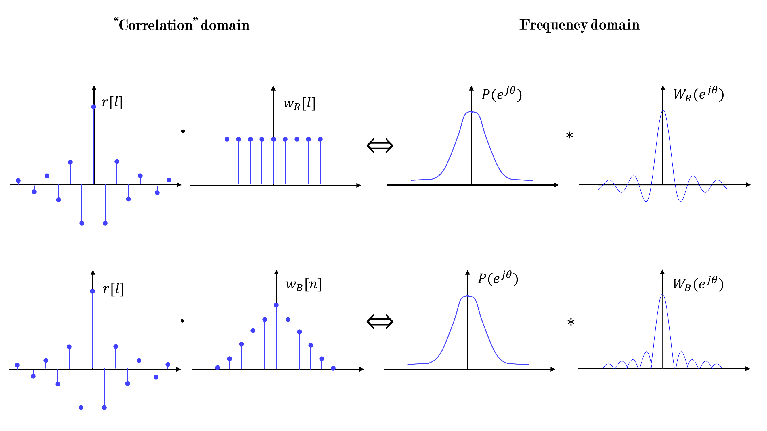
\begin{equation}\label{eq:ac_biased2} \hat{r}_b[l]= r[l] \cdot w_B[l], \end{equation}

\begin{equation}\label{eq:ac_unbiased2} \hat{r}_{ub}[l]= r[l] \cdot w_R[l], \end{equation}

where $r[l]$ is the true autocorrelation function, while \begin{equation} w_R[l] = \begin{cases} 1, & \text{for }|l| < N\newline 0, & \text{otherwise} \end{cases} \end{equation} and \begin{equation} w_B[l] = \begin{cases} \frac{N-|l|}{N}, & \text{for }|l| < N\newline 0, & \text{otherwise} \end{cases} \end{equation}

are rectangular and triangular windows, respectively, applied for lags $-N <l <N$ in the correlation domain. The triangular window is commonly referred to as Bartlett window. Equations (\ref{eq:ac_biased2}) and (\ref{eq:ac_unbiased2}) basically show that the unbiased estimate is equivalent to looking at the true autocorrelation function in a limited window, while the biased estimate provides a bias equivalent to multiplying for a triangular window.

The expected value of the power spectral density estimator

The expected value of $\hat{P}(e^{j\theta})$ can be found as \begin{equation} \begin{split} \mathrm{E}\left[\hat{P}(e^{j\theta})\right] &= \mathrm{E}\left[\sum_{l=-(N-1)}^{N-1} \hat{r}_x[l]e^{-jl\theta}\right], \newline &= \sum_{l=-(N-1)}^{N-1} \mathrm{E}\left[\hat{r}_x[l]\right]e^{-jl\theta}. \end{split}\label{eq:exp_corr} \end{equation}

Using the Wiener-Khinchine relationship in equation (\ref{eq:wiener_k}) and combining equation (\ref{eq:exp_corr}) with eqs. (\ref{eq:ac_biased2}) or (\ref{eq:ac_unbiased2}), we obtain

\begin{equation}\label{eq:expect_win} \mathrm{E}\left[\hat{P}(e^{j\theta})\right] = \sum_{l=-\infty}^{\infty} \mathrm{E} \left[ w[l]r_x[l]e^{-jl\theta} \right], \end{equation}

where $w[l]$ is a generic window function, which is non zero only for $-N<l<N$.

When this relationship is regarded in the Fourier domain the multiplication-convolution property of the Fourier transform should be taken into account. It states that a multiplication in the time domain results in a convolution in the frequency domain. Therefore, the expected value of the estimated PSD function can be interpreted as the (periodic) convolution in the frequency domain between the true power spectral density function and the spectrum of a window function. This convolution is given by \begin{equation}\label{eq:exp_p} \mathrm{E}\left[\hat{P}(e^{j\theta})\right] = P(e^{j\theta})\ast_{2\pi} W(e^{j\theta}) =\frac{1}{2\pi} \int_{-\pi}^{\pi}P(e^{j\theta})W(e^{j(\theta- \phi}))d\phi \end{equation}

This shows that the correlogram (or periodogram) provides an estimate of the power spectral density which is a smoothed version of the true PSD (see Fig. 1). As $N\rightarrow\infty$ the spectrum of the window function will approach a delta pulse function and the expected value of the estimated periodogram will become the true periodogram. In fact, convolving any function with a delta pulse gives the function itself.

From equation (\ref{eq:exp_p}) we also notice that the expected value of the PSD estimator is related to the spectrum of the window function. For a rectangular window, this results in \begin{equation}\label{eq:ft_rect} W_R(e^{j\theta}) = \left(\frac{\sin(N\theta/2)}{\sin(\theta/2)}\right)e^{-j\frac{N-1}{2}\theta}, \end{equation} which is a periodic sinc function (diric).

For a triangular window, we obtain \begin{equation}\label{eq:ft_triang} W_B(e^{j\theta}) = \frac{1}{N}\left(\frac{\sin(N\theta/2)}{\sin(\theta/2)}\right)^2, \end{equation} which is a squared periodic sinc function (squared diric). The proof of (\ref{eq:ft_triang}) is beyond the scope of this reader, but it can easily be found by regarding the Bartlett window as a convolution between two rectangular windows of same length, that is $w_B[n]=w_R[n]\ast w_R[n]$. Then, by the multiplication-convolution property of the Fourier transform, in the frequency domain the result is the multiplication of two rectangul window transform, that is $W_B(e^{j\theta}) =W_R(e^{j\theta})\cdot W_R(e^{j\theta})= $ $= \text{diric}(\theta) \cdot \text{diric}(\theta) = \text{diric}^2(\theta)$.

Since $W_R(e^{j\theta})$ can have negative values, it may lead to an invalid power spectral density function, which by definition is always non-negative. For a triangular window we instead obtain a squared periodic sinc, which is a non-negative function. This explains why we typically use the biased estimate of the autocorrelation function $r_b[l]$ given in (\ref{eq:ac_biased}). In fact, although unbiased, using $r_{ub}[l]$ to estimate the PSD by the correlogram method might lead to an invalid PSD.

As a rule of thumb, it is good to use at least 50 samples and use the biased estimator to calculate on lags up to a quarter of the number of samples.

A key aspect here is that the window is applied directly to the autocorrelation rather than to the signal. Thus, to obtain the PSD estimate, we simply take the transform of the windowed autocorrelation (correlogram), while if we were to calculate the PSD estimate from the signal, we would need to calculate the modulus squared of the transform (periodogram).

Loss of resolution and spectral leakage

In section Windowing, we saw how windowing a signal before calculating the spectrum leads to loss of resolution and spectral leakage. To better understand the contributions of the main and side lobes, let us rewrite the window function as a sum of two components as $W_B(e^{j\theta}) = W_{ML}(e^{j\theta}) + W_{SL}(e^{j\theta})$, with $W_{ML}(e^{j\theta}) $ accounting for the main lobe and given by

\begin{equation} W_{ML}(e^{j\theta}) = \begin{cases} W_B(e^{j\theta}) , & \text{for }|\theta| < \frac{2}{\pi} \newline 0, & \text{otherwise} \end{cases}, \end{equation}

and $W_{SL}(e^{j\theta})$ accounting for the side lobes and given by

\begin{equation} W_{SL}(e^{j\theta}) = W_B(e^{j\theta}) - W_{ML}(e^{j\theta}). \end{equation}

Then, we can rewrite equation (\ref{eq:exp_p}) as \begin{equation}\label{res_leakage} \hat{P}(e^{j\theta}) = \underbrace{P(e^{j\theta})\ast_{2\pi} W_{ML}(e^{j\theta})}_{\text{Loss of resolution}} + \underbrace{P(e^{j\theta})\ast_{2\pi} W_{SL}(e^{j\theta})}_{\text{Spectral leakage}} \end{equation}

From equation (\ref{res_leakage}), we can easily separate the contribution of the main lobe, which causes loss in spectral resolution, from the contribution of the side lobes, which cause spectral leakage, that is the appearance of spurious spectral peaks at the location of the side lobes.

Calculation of the biased auto-correlation function using the DFT (out of scope)

When dealing with windowed signals longer than 100 samples, the auto-correlation function is oftentimes more efficiently calculated using the Discrete Fourier Transform (DFT) or Fast Fourier Transform (FFT). Fig. 2 shows a schematic overview of the calculation procedure. Normally the signal is windowed using a window of length $N$. From this windowed signal the auto-correlation function of length $2N-1$ can be calculated through the definition of the auto-correlation function. Another way of performing this calculation is as follows. First, the signal is windowed with length $N$ and zero-padded to length $M$. The windowed signal should be at least $2N-1$ samples long. From this signal the DFT or FFT is calculated and its magnitude is squared and normalized, after which the inverse DFT (IDFT) or IFFT is calculated. From the obtained signal, the auto-correlation function can be determined by shifting the signal segments as indicated in Fig. 2.

The variance of the power spectral density estimator

The variance of the “raw” PSD estimator (periodogram/correlogram) is rather challenging to calculate since it has dependencies on the fourth-order moment of the signal. In the simple case of an AR(1) process it can be calculated as

\begin{equation}\label{var_ar1} \text{Var}\left[\hat{P}_{AR1}(e^{j\theta})\right] = \sigma_i^2 \left[1 + \left(\frac{1}{N} \frac{\sin(\theta N)}{\sin \theta}\right)^2\right]. \end{equation}

Another simple case is a normally distributed sequence $x[n]$ input to an LTI, for which we obtain \begin{equation}\label{var_gaussin} \text{Var}\left[\hat{P}_{x}(e^{j\theta})\right] = (P(e^{j\theta}))^2\left[1 + \left(\frac{1}{N} \frac{\sin(\theta N)}{\sin \theta}\right)^2\right]. \end{equation}

Although the proof is beyond the scope of this reader, a general trend for the variance of the “raw” PSD estimator can be deducted from equations (\ref{var_ar1}) and (\ref{var_gaussin}): the variance is proportional to the square of the true spectrum. This can be approximately written as

\begin{equation} \text{Var}\left[\hat{P}_{x}(e^{j\theta})\right] \approx (P(e^{j\theta}))^2, \end{equation}

From this it can be seen that $\hat{P}(e^{j\theta})$ is not a consistent estimator, since the variance does not converge to zero for increasing $N$.

Periodogram improvements

When the power spectral density is estimated using the squared Fourier transform of the signal, it is referred to as a periodogram. There exist different methods to improve the “raw” periodogram, which will be discussed hereafter.

Bartlett's method: average periodogram

The periodogram was determined as an asymptotically unbiased, non-consistent estimator of the power spectral density. If the window length goes to $\infty$, the bias reduces, however, the variance does not decrease.

Bartlett proposed a procedure by which the variance can be decreased. He thought of a procedure consisting of averaging the estimated periodograms of smaller signal segments by splitting the total signal of length $N$ into $k$ segments of length $M$. In other words, the original signal $x[n]$ of length $N$ is split into $k$ smaller but equally long non-overlapping signals $x_i[n]$ of length $M$, from which the respective power spectral density estimators can be written as \begin{equation} \hat{P}_i(e^{j\theta}) = \frac{1}{M}\left|\sum_{n=0}^{M-1} x_i[n]e^{-jn\theta}\right|^2. \qquad \text{for }i=1,2,\ldots,k \end{equation} The final power spectral density estimator can then be determined by averaging all the sub-periodograms as \begin{equation} \hat{P}_B(e^{j\theta}) = \frac{1}{K} \sum_{i=1}^K \hat{P}_i(e^{j\theta}). \end{equation} Fig. 3 shows a graphical representation of the described method.

To understand why this method actually decreases the variance, we first take a look at the estimator expected value. The expected value can be determined as \begin{equation} \begin{split} \mathrm{E}\left[\hat{P}_B(e^{j\theta})\right] &= \mathrm{E}\left[\frac{1}{K} \sum_{i=1}^K \hat{P}_i(e^{j\theta})\right], \newline &= \frac{1}{K} \sum_{i=1}^K\mathrm{E}\left[ \hat{P}_i(e^{j\theta})\right], \newline &= \mathrm{E}\left[ \hat{P}(e^{j\theta})\right], \newline &= \frac{1}{2\pi} P(e^{j\theta})\ast W_B(e^{j\theta}), \end{split} \end{equation} which indeed shows a similar relationship as obtained previously; however, because the signal segments are now shorter ($M<N$) the bias increases because of poorer estimation of the auto-correlation function in (\ref{eq:autocorr_est}), which is calculated on a smaller number of samples. On the other hand, the variance can be determined as \begin{equation} \begin{split} \text{Var}\left[\hat{P}_B(e^{j\theta})\right] &= \text{Var}\left[\frac{1}{K} \sum_{i=1}^K \hat{P}_i(e^{j\theta})\right], \newline &= \frac{1}{K^2}\text{Var}\left[ \sum_{i=1}^K \hat{P}_i(e^{j\theta})\right], \newline &= \frac{1}{K}\text{Var}\left[ \hat{P}_i(e^{j\theta})\right] \approx \frac{1}{K} P(e^{j\theta})^2, \end{split}\label{eq:bartlett} \end{equation} which proves that the variance indeed decreases for an increase in the number of signal segments. From this it can be concluded that Bartlett's method reduces the variance of the periodogram at the cost of an increased bias.

Welch's overlapped segment averaging (WOSA) method

A similar method is Welch's method, also known as Welch's overlapped segment averaging (WOSA) spectral density estimation. In this method, the signal is also split in different segments but now allowing overlapping between the segments (typically with 50% or 75% overlap); then these segments are windowed before calculating the individual periodograms, and then averaged, similarly to Bartlett's method. Fig. 3 shows a graphical visualisation of this method. The consequence of this overlap is that the individual segments are now no longer independent, which results in (\ref{eq:bartlett}) not being valid anymore. When applying this method the variance is still decreased, but to a smaller extent compared to Bartlett's method. On the other hand, since the segments are now longer due to the overlap, the bias does not increase as much as with Bartlett's method.

Correlogram improvements

When the power spectral density is estimated using the Fourier transform of the estimated auto-correlation function, it is referred to as a correlogram. Hereafter, we describe an improvement known as the Blackman-Tukey correlogram.

Blackman-Tukey method

The basic idea of The Blackman-Tukey correlogram is to apply a symmetric window function $w_M[n]$ of length $2M-1$ to the estimated auto-correlation function. The Blackman-Tukey estimate of the power spectral density $\hat{P}_{BT}(e^{j\theta})$ can be defined as \begin{equation} \hat{P}_{BT}(e^{j\theta}) = \sum_{l=-(M-1)}^{M-1} w_M[l]\hat{r}[l]e^{-jl\theta}. \end{equation} Here the estimated auto-correlation function is windowed. Note that window is additional to the triangular window which is inherent in the biased estimation of the autocorrelation function. The reason to include an extra window is due to the fact that the estimated auto-correlation is very uncertain at the edges of the observation window, since at these lags it is calculated using a very limited number of samples. Whereas in the center of the window $\hat{r}[l]$ is computed with almost all samples available. Therefore, by using a suitable window, we can reduce the weight of the auto-correlation lags at the edges of the window, where only few samples are available. In the frequency domain, the Blackman-Tukey estimator can be interpreted as the convolution between the spectrum of the window and the estimated power spectral density as \begin{equation} \hat{P}_{BT}(e^{j\theta}) = \frac{1}{2\pi} \hat{P}(e^{j\theta})\ast W_M(e^{j\theta}). \end{equation} Let us now determine the performance of this method. The expected value of the estimator can be determined using (\ref{eq:exp_p}) as \begin{equation} \begin{split} \mathrm{E}\left[\hat{P}_{BT}(e^{j\theta})\right] &= \frac{1}{2\pi}\mathrm{E}\left[\hat{P}(e^{j\theta})\right] \ast W_M(e^{j\theta}), \newline &= \frac{1}{2\pi} P(e^{j\theta})\ast W_B(e^{j\theta})\ast W_M(e^{j\theta}), \newline &\approx \frac{1}{2\pi} P(e^{j\theta})\ast W_M(e^{j\theta}), \end{split} \end{equation} where it is assumed that the Blackman-Tukey window has a length significantly smaller than the length of the auto-correlation function. This assumption also results in the spectrum of the Blackman-Tukey window having wider lobes in comparison to the spectrum of the Bartlett window, which was a direct consequence in the definition of the auto-correlation estimator. Using the definition of the continuous convolution in the frequency domain, the expected value of the estimator can be rewritten as \begin{equation} \mathrm{E}\left[\hat{P}_{BT}(e^{j\theta})\right] \approx \frac{1}{2\pi} \int_{-\pi}^\pi P(e^{j\phi})W_M(e^{j(\theta-\phi)})\mathrm{d}\phi. \end{equation} If we now were to consider the window for an increasing length $2M-1$, we would find \begin{equation}\label{eq:windlim} \lim_{M\rightarrow\infty} W_M(e^{j\theta}) = A\delta(\theta), \end{equation} which states that the frequency spectrum of the window function converges to a delta pulse. Thus $\hat{P}_{BT}(e^{j\theta})$ is unbiased provided that $A=1$. This occurs if \begin{equation} \frac{1}{2\pi} \int_{-\pi}^\pi W_M(e^{j(\theta)})\mathrm{d}\theta = \frac{1}{2\pi} \int_{-\pi}^\pi A\delta(\theta) \mathrm{d}\theta = 1 = w_m[0], \end{equation} where the latter passage is due to the basic properties of the Fourier transform. Combining the previous two equations leads to \begin{equation} \mathrm{E}\left[\hat{P}_{BT}(e^{j\theta})\right] \approx P(e^{j\theta}) \frac{1}{2\pi} \int_{-\pi}^\pi A\delta(\theta) \mathrm{d}\theta = w_M[0] P(e^{j\theta}) \end{equation} stating that the estimator is asymptotically unbiased if $A=1$ or equivalently $w_M[0] =1$. Note that the approximation is only valid in the assumption of very large $M$. In this case the main lobe of the window is so narrow, that we can consider $P(e^{j\theta})$ constant within the narrow main-lobe.

The variance of the Blackman-Tukey estimator can be found as \begin{equation} \text{Var}\left[\hat{P}_{BT}(e^{j\theta})\right] \approx \frac{P(e^{j\theta})^2}{N}\left(\sum_{l=-(M-1)}^{M-1} w_m^2[l]\right), \end{equation} which shows that the estimator is consistent when $N \rightarrow \infty$. There is a compromise made for the length of the Blackman-Tukey window function $M$. A large value of $M$ will namely decrease the bias of the estimator, since the spectrum of the window will approach a delta pulse, and the variance of the estimator will increase, because of the longer summation, including more lags at the edges (more uncertain).

Methods summary

The “raw” periodogram and correlogram calculate the power spectral density by either the square of the absolute windowed signal spectrum or by the Fourier transform of the estimated auto-correlation function, respectively. They produce asymptotically unbiased estimators for an increasing length of the signal. However, there is no way to decrease the variance.

Bartlett's method improves the “raw” periodogram by averaging over multiple power spectral density estimators, which are calculated for non-overlapping segments of the signal. Using this approach the variance can be decreased by using more segments, but the bias is increased.

Welch's method is similar to Bartlett's method, but allows for overlap between the windowed segments. Because the estimators are no longer independent, the variance does not decrease as much, but neither will the bias increase as much.

Blackman-Tukey (BT) method uses a different approach and windows the auto-correlation estimator, because this estimator contains a lot of uncertainty around its borders due to the limited number of samples used to calculate the auto-correlation at these points. This can be seen in the Fourier domain by convolving the estimated power spectral density (which is already a convolution between the true power spectral density and a triangular window for the biased estimator) with the spectrum of the BT window function. A longer window allows for more uncertainty, increasing the variance, but reduces the effects of the convolution, therefore decreasing the bias.

Fig. 4 shows the estimated power spectral density of the signal \begin{equation} x[n] = \cos(0.35\pi n) + \cos(0.4\pi n) + 0.25\cos(0.8 \pi n) + \epsilon[n], \end{equation} where $\epsilon[n]$ is standard Gaussian noise. In this figure several methods are used to estimate the power spectral density using various design parameters. Please note the important differences and characteristics of each method and see how the parameters affect the spectral estimation. In the figure, the BT window length is denoted by $L$ instead of $M$.