A stochastic process may be represented by a stochastic model with given order and parameters, which is able to generate a random signal characterized by well-defined spectral properties. Signal modeling is closely related to spectral factorization which states that most random processes with a continuous power spectral density (PSD) can be generated as the output of a causal filter driven by white noise, the so-called innovation representation of the random process. In this section, we first explain how the statistical properties of a random signal are affected when filtering by a LTI system; then we discuss random signals with rational spectra and an important representation of a random signal known as the innovation representation; finally we explain how spectral factorization can be used to provide the innovation representation of a random signal.
LTI with random inputs
When a random signal is filtered by an LTI system, its statistical properties are changed. Focusing on the second-order statistics, here we show the transformation that a discrete random power signal undergoes when processed by a discrete-time LTI system. The difference between power and energy signal is discussed in the section Power Spectral Density.
Screencast video [⯈]
Time-domain analysis
The input-output relationship of an LTI system is described using the following convolution \begin{equation}\label{eq:1} y[n] = \sum_{k=-\infty}^{\infty} h[k] x[n-k]. \end{equation} Here $x[n]$ is a random stationary signal. Output $y[n]$ converges and is stationary if the system represented by the impulse response $h[k]$ is stable. The condition for stability is that $\sum_{-\infty}^{\infty}|h[k]|<\infty$.
The exact output $y[n]$ cannot be calculated, since $y[n]$ is a stochastic process. However, certain statistical properties of $y[n]$ can be determined from knowledge of the statistical properties of the input and the characteristics of the system.
The mean value of output $y[n]$ can be determined by taking the expected value from both sides of equation (\ref{eq:1}) as \begin{equation} \begin{split} \mu_y = \sum_{k=-\infty}^{\infty}h[k]E\{{x[n-k]}\} = \mu_x \sum_{k=-\infty}^{\infty} h[k] = \mu_x H(e^{j0}). \end{split} \end{equation} Note that the filter coefficients are deterministic, and thus $E\{h[k]\} = h[k]$.
The input-output correlation can also be calculated without knowing the exact output. The input-output correlation is defined as $r_{xy}[l] = E\{ x[n+l]y^\ast[n]\}$. Therefore, to calculate this correlation, we take the complex conjugate of (\ref{eq:1}) and multiply it with $x[n+l]$ before taking the expected value.
\begin{equation} \begin{split} r_{xy}[l] &= E\{ x[n+l]y^\ast[n]\} = \sum_{k=-\infty}^{\infty} h^\ast[k] E\{x[n+l]x^\ast[n-k]\}\newline r_{xy}[l] &= \sum_{k=-\infty}^{\infty} h^\ast[k] r_{xx}[l+k] = \sum_{m=-\infty}^{\infty} h^\ast[-m] r_{xx}[l-m]\newline r_{xy}[l] &= h^\ast[-l]\star r_{xx}[l]\newline r_{yx}[l] &= h^\ast[l]\star r_{xx}[l].\newline \end{split} \end{equation}
The output correlation can be calculated by multiplying with $y^\ast[n-l]$ and taking the expectation. \begin{equation} \begin{split} r_{yy}[l] &= E\{y[n]y^\ast[n-l]\} = \sum_{k=-\infty}^{\infty} h[k]E\{x[n-k] y^\ast[n-l]\}\newline r_{yy}[l] &= \sum_{k=-\infty}^{\infty} h[k] r_{xy}[l-k] = h[l]\star r_{xy}[l]. \end{split} \end{equation}
By combining this result with $r_{xy}[l] = h^\ast[-l]\star r_{xx}[l]$ we obtain \begin{equation} \begin{split} r_y[l] &= h[l]\star h^\ast[-l]\star r_x[l]\newline r_y[l] &= r_h[l]\star r_x[l], \end{split} \end{equation} where $r_h[l]$ is the autocorrelation of the LTI system with inmpulse response $h[n]$.
The output signal power is equal to $P_y=E{|y[n]|^2}=r_y[0]$, which can be calculated using the previous equations, \begin{equation} \begin{split} P_y&=E{|y[n]|^2}=r_y[0]\newline &=r_h[l]\star r_x[l=0] = \sum_{k=-\infty}^{\infty} h[k] h^\ast[-k] r_{x}[k]. \end{split} \end{equation}
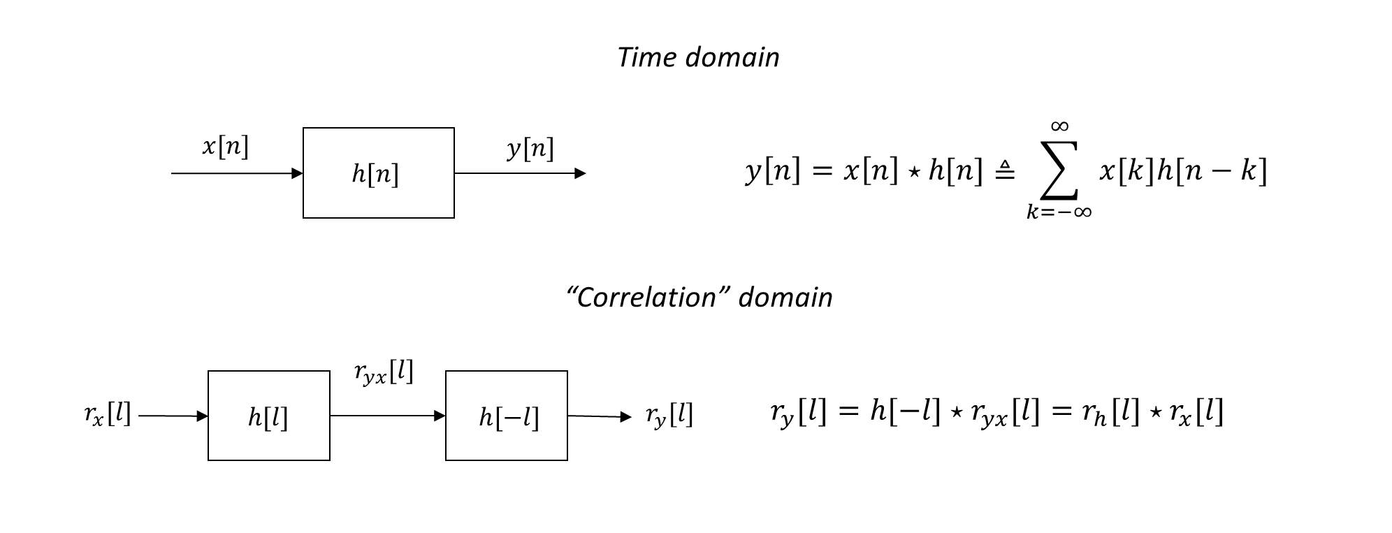
Figure 1 describes schematically what the input-output relationship of an LTI system in the time domain and in the “correlation” domain.
Transform-domain analysis
The relationships found above in the time domain can be easily transformed in the frequency- and z-domains. Let us first recall some properties of the z-transform. Given a complex sequence $x[n]$, with z-transform $X(z)$, the following properties apply \begin{equation} \begin{split} x^\ast[n] \Longleftrightarrow & X^\ast(z^\ast) \newline x[-n] \Longleftrightarrow & X(1/z) \newline x^\ast[-n] \Longleftrightarrow & X^\ast(1/z^\ast) \newline \end{split} \end{equation}
Since we are dealing with autocorrelation functions and power spectral densities of mostly real signals, it is also useful to recall that
- if $x[n]$ is real, then \begin{equation} x[n] = x^\ast[n] \Longleftrightarrow X(z) = X^\ast(z^\ast); \end{equation}
- if $x[n]$ has even symmetry around the time origin, then \begin{equation} x[n] = x[-n] \Longleftrightarrow X(z) = X(1/z); \end{equation}
- if $x[n]$ is both real and even, then \begin{equation} x[n] = x^\ast[-n] \Longleftrightarrow X(z) = X^\ast(z^\ast) = X(1/z) = X^\ast(1/z^\ast). \end{equation}
Using the above properties, we can easily calculate the input-output relationships for an LTI system in the frequency and z-domain, which are provided in the following table.
| Time Domain | Frequency domain | z-domain |
|---|---|---|
| $y[n]=h[n]\star x[n]$ | $Y(e^{j\theta})=H(e^{j\theta})X(e^{j\theta})$ | $Y(z)=H(z)X(z)$ |
| $r_{yx}[l]=h[l]\star r_x[l]$ | $P_{yx}(e^{j\theta})=H(e^{j\theta})P_{x}(e^{j\theta})$ | $P_{yx}(z)=H(z)P_{x}(z)$ |
| $r_{xy}[l]=h^*[-l]\star r_x[l]$ | $P_{xy}(e^{j\theta})=H^*(e^{j\theta})P_{x}(e^{j\theta})$ | $P_{xy}(z)=H^*(1/z^*)P_{x}(z)$ |
| $r_{y}[l]=h[l]\star r_{xy}[l]$ | $P_{y}(e^{j\theta})=H(e^{j\theta})P_{xy}(e^{j\theta})$ | $P_{y}(z)=H(z)P_{xy}(z)$ |
| $r_{y}[l]=h[l]\star h^*[-l]\star r_x[l]$ | $P_{y}(e^{j\theta})=|H(e^{j\theta})|^2P_{x}(e^{j\theta})$ | $P_{y}(z)=H(z)H^*(1/z^*)P_{x}(z)$ |
Innovation representation of a random signal
A rational spectrum is a ratio of two rational functions containing $e^{j\theta}$. \begin{equation} \begin{split} P(e^{j\theta}) = P(z) = \frac{\sum_{q=-Q}^{Q} \gamma_1[q] e^{-j\theta q}}{\sum_{p=-P}^{P} \gamma_2[p] e^{-j\theta p}} \end{split} \end{equation}
Here $\gamma_1[q]$ and $\gamma_2[p]$ are two series with even symmetry, similarly to the auto-correlation sequences of real signals. The rational spectrum is actually derived from the Wold's decomposition or representation theorem, a very general signal decomposition theorem, which states that every WSS signal can be written as the sum of two components, one deterministic and one stochastic, as given below \begin{equation}\label{eq:xnlti} x[n] = \sum_{k=0}^{\infty}h[k]w[n-k] + y[n], \end{equation}
where $h[k]$ represents a infinite-length sequence of weights; $w[n]$ is a signal of uncorrelated samples, often referred to as innovations; $y[n]$ is deterministic, thus exactly predictable from the past values. The deterministic part can be subtracted from this signal since it is exactly predictable.
Let us know consider a purely zero-mean WSS signal, from which any deterministic component has already been subtracted. We take a white noise sequence, $i[n]$, as the uncorrelated samples. Then Wold's decomposition theorem becomes
\begin{equation}\label{eq:reversesum} x[n] = \sum_{k=0}^{\infty}h[k] i[n-k] = \sum_{k=-\infty}^{n}h[n-k] i[k]. \end{equation}
The sequence of weights $h[k]$ can now be seen as the samples of the impulse response of a causal LTI filter, which we require to be stable. We also assume this filter to have a rational transfer function of the form
\begin{equation} \begin{split} H(z) = \frac{B(z)}{A(z)}, \end{split} \end{equation} with \begin{eqnarray}\label{#eq:AB} A(z) &=& 1 + a_1z^{-1}+ … + a_pz^{-p},\newline B(z) &=& 1 + b_1z^{-1}+ … + b_qz^{-q} \nonumber. \end{eqnarray} In equation (\ref{#eq:AB}), we assume that $a_0 = 1$ and $b_0 = 1$. Note that this is not too restrictive. In fact, according to the rational approximation of function, we can always approximate any continuous function by a rational polynomial as closely as we want by increasing the degree of the numerator and denominator in (\ref{#eq:AB}). However, the poles of the transfer function must be inside the unit circle for the filter to be stable.
In summary, Wold's decomposition theorem allows us to represent any WSS random signal as the output of an LTI filter driven by white noise. If the filter has transfer function $H(z) = B(z)/A(z)$, then the signal can be rewritten as \begin{equation} \begin{split} x[n] = -\sum_{p=1}^{p}a_p x[n-p] + \sum_{q=0}^{Q}b_q i[n-q]. \end{split} \end{equation} Since the input is given by a white-noise sequence, the input autocorrelation is of the form $r_i[l] = \sigma_i^2 \delta[l]$. Given that the transfer function is rational, also the power spectrum of the output random signal is rational, and can be calculated as \begin{equation}\label{eq:psdlti} P_{x}(e^{j\omega}) = \sigma_i^2 \frac{|B(e^{j\omega})|^2}{|A(e^{j\omega})|^2} = \sigma_i^2 |H(e^{j\omega})|^2, \end{equation} where \begin{equation} \begin{split} A(e^{j\omega}) = 1 + a_1e^{-j\omega} + … + a_p e^{-j \omega p}, \newline B(e^{j\omega}) = 1 + b_1e^{-j\omega} + … + b_q e^{-j \omega q}. \end{split} \end{equation}
As we shall see in the section Auto-regressive moving-average (ARMA) signal models , this means viewing an observed random signal as a stochastic process modeled by an auto-regressive moving-average (ARMA) process, whose rational spectrum contains the model parameters.
Spectral factorization
Screencast video [⯈]
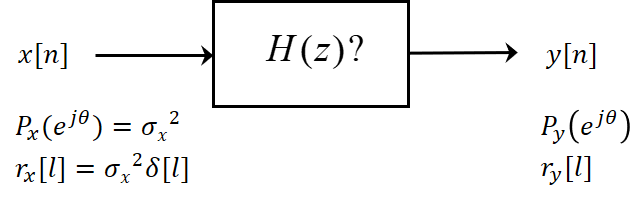
In the module Power spectral density, we have seen that the PSD and the AC of a random signal are Fourier pairs. Consider the system depicted in Figure 1, with input $x[n]$ and output $y[n]$.
Spectral factorization tackles the following question: Can we determine $H(z)$ knowing that the input $x[n]$ is white noise, and given the second-order statistics ($r_y[l]$ or equivalently $P_y(e^{j\theta})$) of the output signal $y[n]$? In principle, there is no unique answer to this question. We can see this by considering the following example.
Suppose we are given the PSD of $y[n]$ as $P_y(e^{j\theta}) =\frac{5}{4}-cos(\theta)$ and we know that $y[n]$ is the output of an LTI system driven by white noise, with zero mean and variance $\sigma_i^2$. Based on equation (\ref{eq:psdlti}), we can write: \begin{equation*} \begin{split} P_y(e^{j\theta}) &=& \sigma_i^2|H(e^{j\theta})|^2 = \frac{5}{4}-cos(\theta)\newline \sigma_i^2|H(z)|^2 &=& \sigma_i^2H(z)H(z^{-1}) = \frac{5}{4}-\frac{z+z^{-1}}{2}\newline \end{split} \end{equation*}
Knowledge of $P_y(e^{j\theta})$ provides us with the magnitude response of the system, i.e. $|H(z)|$. However, there are two possible cases which provide the same magnitude response $|H(z)|^2$:
- In the first case, we can define $H(z)$ and the input noise variance as: \begin{equation*} H(z) = 1-\frac{1}{2}z^{-1}, \quad \text{with} \quad \sigma_i^2=1. \end{equation*} This choice gives as output $P_y(e^{j\theta})$, as proven below: \begin{equation*} \begin{split} \sigma_i^2 H(z)H(z^{-1})&=& (1-\frac{1}{2}z^{-1})(1-\frac{1}{2}z)\newline & =& 1-\frac{z+z^{-1}}{2}+\frac{1}{4} = \frac{5}{4}-\frac{z+z^{-1}}{2}\newline \end{split} \end{equation*}
- Alternatively, we can define $H(z)$ and the input noise variance as: \begin{equation*} H(z) = 1-2z^{-1}, \quad \text{with} \quad \sigma_i^2=\frac{1}{4}. \end{equation*} This choice gives the same output $P_y(e^{j\theta})$, as proven below: \begin{equation*} \begin{split} \sigma_i^2 H(z)H(z^{-1})&=& \frac{1}{4}(1-2z^{-1})(1-2z)\newline & = &\frac{1}{4}-\frac{z+z^{-1}}{2}+1 = \frac{5}{4}-\frac{z+z^{-1}}{2}\newline \end{split} \end{equation*}
Therefore, more constraints are needed to uniquely define $H(z)$ which gives $r_y[l]$ or $P_y(e^{j\theta})$.
Spectral factorization is defined as the determination of a minimum-phase system from its magnitude response or from its auto correlation function. If $P(z)$ is rational, it can be factorized in the following form $\sigma_i^2 L(z)L(z^{-1})$, in which the so-called “innovation filter” $L(z)$ is minimum-phase, and $\sigma^2_i$ is chosen such that $l[0]=1$.
One practical method to solve the spectral factorization problem is referred to as the root method. The basic principles are:
- For every rational PSD, that is a PSD that can be expressed as a fraction between two polynomials in $e^{j\omega}$ (or equivalently in $z$), there exists a unique minimum-phase factorization within a scale factor.
- For a PSD expressed as a rational polynomial, with a numerator of order Q and a denominator of order P, there are $2^{P+Q}$ possible rational systems which provide this PSD.
- Not all possible rational systems are valid, since for a valid PSD the roots should appear in mirrored pairs, which means that if $z_k$ is a root, then also $1/z^\ast_k$ is a root.
In the example above, we therefore need to choose $H(z) = 1-\frac{1}{2}z^{-1}$ because it is the minimum-phase choice.
Pencast video [⯈]
In the following pencast, you may see how to find the spectral factorization of a random signal by the root method.
In the following exercise, you can try using the root method to find the spectral factorization of a random signal.
Exercise
Apply spectral factorization to the following PSD: \begin{equation*} P(e^{j\theta}) = \frac{5-4 \cos(\theta)}{10-6 \cos(\theta)} \end{equation*} Give an expression for the innovation filter $L(z)$ and the variance $\sigma^2_i$ of the innovation signal.
From above, we obtain the following set of equation: \begin{equation*} \begin{split} c_n (1-a z^{-1}) (1-az) &=& 5 -2(z^{-1}+z) \mbox{ } \newline &\Rightarrow & (a=\frac{1}{2} \mbox{ and } c_n =4) \mbox{ or } (a=2 \mbox{ and } c_n =1) \newline c_d (1-b z^{-1}) (1-b z) &=& 10 -3(z^{-1}+z) \mbox{ } \newline &\Rightarrow & (b=\frac{1}{3} \mbox{ and } c_d =9) \mbox{ or } (b=3 \mbox{ and } c_d =1) \end{split} \end{equation*} Since we need to choose that solution which results in a minimum phase innovation filter, this results in: \begin{equation*} P(z) = \frac{4}{9} \cdot \left ( \frac{1- \frac{1}{2} z^{-1}}{1- \frac{1}{3} z^{-1}} \right ) \cdot \left ( \frac{1- \frac{1}{2} z}{1- \frac{1}{3} z} \right ) = \sigma_{i}^{2} \cdot L(z) \cdot L(z^{-1}) \end{equation*} Thus $L(z) = (1- \frac{1}{2} z^{-1})/(1- \frac{1}{3} z^{-1})$ and $\sigma_{i}^{2} = 4/9$.