Introduction
The application of the least-squares estimation dates back until Gauss, who used it to study planetary motions. The popularity of the least-squares estimation has not decreased ever since and it remains a widely applied estimator. The least-squares estimator (LSE) does not make any probabilistic assumptions on the observed data. Thus, it is suitable in situations where the precise statics is not known. However, due to the lack of statics of the observed data, no assertion about optimality of the estimator can be made.
The concept of the least-squares estimation can be described as follows. A signal is generated by a deterministic signal model $s[n;\theta]$ that is parametrized by a parameter $\theta$. Due to noise or model inaccuracies, the observed data $x[n]$ deviates from the signal model. As the name suggest, the least-squares approach aims to minimize the squared difference between the observed data and the signal model. Thus, the least-squares error criterion is defined as \begin{equation} J(\theta) = \sum_{n=0}^{N-1}(x[n]-s[n;\theta])^2. \label{eq:ls_criterion} \end{equation}
The least-squares estimate $\hat{\theta}_{\text{LSE}}$ is the value of the parameter $\theta$ that minimizes \eqref{eq:ls_criterion}, i.e., \begin{equation} \hat{\theta}_{\text{LSE}} = \underset{\theta}{\operatorname{arg\,min}}J(\theta). \end{equation} From this perspective, the least-squares estimator can be considered as an optimization problem of fitting a model to some available data.
Example:
Suppose we want to estimate the energy consumption per km of an electric car. For this pupose, we record at each recharge of the car the amount of energy charged $E$ and the distance travelled $D$. Visualizing the recordings give following picture.
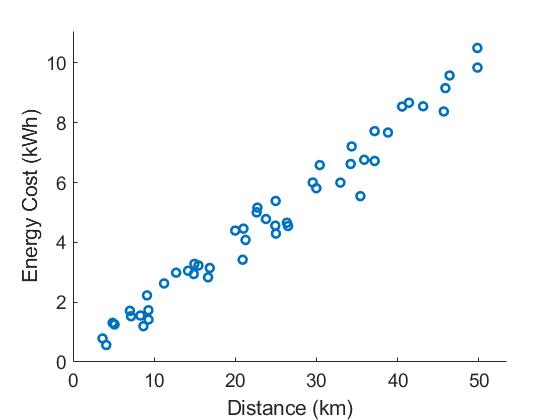
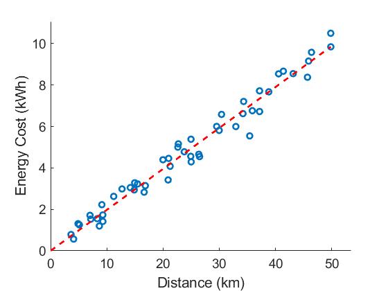
From the figure we can see that the energy consumption increases almost linearly with the distance travelled. Thus, we can assume a linear relation between the energy consumption and the distance travelled: \begin{equation} s[n;\theta] = \theta D[n]. \label{eq:model} \end{equation} In this model, the parameter $\theta$ represents the slope of the line. From the figure, however, we can also see that the data points do not exactly lie on a line. The discrepancy between the model and data comes from the model inaccuracy: the energy consumption depends on more parameters than just the distance. Nonetheless, the suggest model serves our purpose. The least-square error criterion becomes \begin{equation} J(\theta) = \sum_{n=0}^{N-1} (x[n]-\theta D[n])^2. \end{equation} Taking the derivative with respect to $\theta$ and equating it to zero yields \begin{equation} \hat{\theta}_{\text{LSE}} = \frac{\sum_{n=0}^{N-1}x[n]D[n]}{\sum_{n=0}^{N-1}D^2[n]}. \label{eq:electric_car} \end{equation}
In the example above, we were only interested in estimating a single parameter $\theta$. In general, the signal model can be dependent on several parameters. Consider for example, the signal model
\begin{equation}
s[n; A, f_0] = A\cos(2\pi f_0 n)
\end{equation}
where $A$ and $f_0$ are the amplitude and the frequency of the signal, respectively. This signal model is parametrized by two parameters $A$ and $f_0$, which can be expressed in a vector $\boldsymbol\theta = [A, f_0]^T$. In this case we write $s[n;\boldsymbol\theta]$. In the following, we will consider vector parameters since the scalar case arise as a special case of the vector parameters.
Depending on the signal model, we can distinguish between linear and nonlinear least-squares estimators. The electric car example was a linear estimation problem, whereas the signal model \begin{equation} s[n,f_0] = A \cos(2\pi f_0 n) \end{equation} is nonlinear in the parameter $f_0$. The focus of this module is the linear LSE. Nonlinear LSE rely on numerical methods which are treated separately in the module Numerical Methods. However, for some particular nonlinear problems it is possible tor convert them either into a linear problem or to separate them into a linear and a nonlinear part. These two special cases are covered at the end of this module.
Linear Least Squares Estimator
A linear signal model, as shown in the module on MVUE for linear signal models, is any model of the form \begin{equation} s[n;\boldsymbol\theta] = \sum_{k=0}^{K-1} h_k[n]\theta_k. \end{equation} Typically, more than one observation is available. In this case, the linear least-squares estimator can be expressed as \begin{equation} \mathbf{s} = \mathbf{H}\boldsymbol\theta \label{eq:ls_linear} \end{equation} where $\mathbf{s}$ is the signal vector, $\mathbf{H}$ is the so called observation matrix, and $\boldsymbol\theta$ is the parameter vector.
Using the matrix notation in \eqref{eq:ls_linear}, the least-squares error criterion in \eqref{eq:ls_criterion} can be expressed as \begin{align} J(\boldsymbol\theta)&= \|\mathbf{x}-\mathbf{H}\boldsymbol\theta\|^2\nonumber\newline &=(\mathbf{x}-\mathbf{H}\boldsymbol\theta)^T(\mathbf{x}-\mathbf{H}\boldsymbol\theta)\nonumber\newline &= (\mathbf{x}^T-\boldsymbol\theta^T\mathbf{H^T})(\mathbf{x}-\mathbf{H}\boldsymbol\theta) \nonumber \newline &= \mathbf{x}\mathbf{x}^T - 2 \mathbf{x}^T \mathbf{H}\boldsymbol\theta +\boldsymbol\theta^T\mathbf{H}^T \mathbf{H}\boldsymbol\theta. \end{align} The corresponding gradient is \begin{equation} \frac{\partial J(\boldsymbol\theta)}{\partial \boldsymbol\theta} = -2\mathbf{H}^T\mathbf{x}+2\mathbf{H}^T\mathbf{H}\boldsymbol\theta. \end{equation} The minimum can be found by setting the gradient to zeros and solving for $\boldsymbol\theta$. The linear least-squares estimator is then \begin{equation} \hat{\boldsymbol\theta}_{\text{LSE}} = (\mathbf{H}^T\mathbf{H})^{-1} \mathbf{H}^T \mathbf{x}, \label{eq:LSE} \end{equation} which is referred to as normal equation. Returning to the electric car example, we have the special case of a single parameter $\theta$. In this case, the observation matrix becomes a vector with the distances $D[n]$ as its entries. The expression $\mathbf{H}^T\mathbf{H} = \sum_{n=0}^{N-1}D^2[n]$. Note that $\sum_{n=0}^{N-1}D^2[n]$ is a scalar and its inverse is $1/(\sum_{n=0}^{N-1}D^2[n])$. On the other hand, the expression $\mathbf{H}^T\mathbf{x}$ is $\sum_{n=0}^{N-1}x[n]D[n]$. Combining these two expressions we obtain the least-squares estimate in \eqref{eq:electric_car}.
Geometric Interpretation
The previous derivation is based on minimizing the squared error term in \eqref{eq:ls_criterion}. The least-square estimation can also be derived based on geometrical interpretations. To obtain this geometrical interpretation, we assume that more observations than parameters to be estimated are available, i.e., $N>K$. With this assumption, we can interpret \eqref{eq:ls_linear} from a geometric point of view. The vector $\mathbf{s}$ and the column space of $\mathbf{H}$ have dimension $N$. However, since $N>K$, the linear combination \begin{equation} \mathbf{s} = \mathbf{H}\boldsymbol\theta = \sum_{k=0}^{K-1} \theta_k \mathbf{h}_k, \end{equation} where $\mathbf{h}_k$ is the $k$th column of $\mathbf{H}$, spans only a $K$ dimensional subspace of the $N$-dimensional space. This is examplified in the next figure for the case $N=3$ and $K=2$.

From the geometric point of view, the least-squares error criterion in \eqref{eq:ls_linear} describes the length of the error vector, i.e., the vector between data vector $\mathbf{x}$ and the $\mathbf{s}$ which is in the subspace. The length of the error vector becomes a minimum if it is orthogonal to the subspace, which is known as the orthogonality principle. An example of an orthogonal error vector is illustrated below.

The error vector is orthogonal to the subspace if it is orthogonal to all vectors which span the space, i.e., \begin{align} \mathbf{H}^T \mathbf{e} = \mathbf{H}^T (\mathbf{x-H}\boldsymbol\theta) = \mathbf{0} \end{align} with $\mathbf{0}$ denoting the zero vector.
\begin{equation} \hat{\boldsymbol\theta}_{\text{LSE}} = (\mathbf{H}^T\mathbf{H})^{-1}\mathbf{H}^T\mathbf{x} \end{equation}
Weighted Least Squares Estimation
For some estimation problems, we might want to reduce the influence of a portion of the data on our final estimate. For example, the data of the can be provided by different sensors. Moreover, some sensors may have a higher accuracy than others, and thus, we have more confidence in their measurement result. However, even though the other sensor measurement results are less accurate, they still provide some information. The different confidence in the measurement result can be incooperated in least-squares estimator by assigning them different weights, which leads to the weighted least-squares estimator (WLSE). In general, we can express the weighted least-squares error criterion as \begin{equation} J(\boldsymbol\theta) = (\mathbf{x}-\mathbf{H}\boldsymbol\theta)^T\mathbf{W}(\mathbf{x}-\mathbf{H}\boldsymbol\theta) \end{equation} where $\mathbf{W}$ is a positive definite matrix. For the particular case that $\mathbf{W}$ is diagonal, we obtain \begin{equation} J(\boldsymbol\theta) = \sum_{n=0}^{N-1} w_n (x[n]-s[n;\boldsymbol\theta])^2, \end{equation} where $w_n$ is the $n$th diagonal element of $\mathbf{W}$.
The weighted LSE is obtained by setting the gradient to zero, which yields \begin{equation} \hat{\boldsymbol\theta}_{\text{LSE}}=(\mathbf{H}^T\mathbf{W}\mathbf{H})^{-1}\mathbf{H}^T\mathbf{W}\mathbf{x}. \end{equation}
Gauss-Markov Theorem
The Gauss-Markov theorem states that if the signal model is linear with additive noise, i.e., \begin{equation} \mathbf{x} = \mathbf{H}\boldsymbol\theta + \mathbf{w}, \end{equation} where $\mathbf{w}$ has zero mean and covariance matrix $\mathbf{C}$, then the WLSE with weights $\mathbf{W} = \mathbf{C}^{-1}$ is the BLUE. The BLUE is then \begin{equation} \hat{\boldsymbol\theta}_{\text{LSE}}=(\mathbf{H}^T\mathbf{C}^{-1}\mathbf{H})^{-1}\mathbf{H}^T\mathbf{C}^{-1}\mathbf{x}, \label{eq:GM} \end{equation} and the covariance matrix is \begin{equation} \mathbf{C}_{\hat{\boldsymbol\theta}} = \left( \mathbf{H}^T\mathbf{C}^{-1} \mathbf{H} \right) ^{-1}. \end{equation} The variance of the individual estimates is given by the diagonal elements of the covariance matrix. Note that the theorem does not specify the actually distribution of the noise. Furthermore, if $\mathbf{C} = \sigma^2\mathbf{I}$, i.e., the noise is uncorrelated and has variance $\sigma^2$, then \eqref{eq:GM} simply is the LSE in \eqref{eq:LSE}
Nonlinear Least Squares Estimator
Until now, we dealt with linear signal models, i.e., functions that are linear in the parameter vector $\boldsymbol\theta$. For this particular case, we were able to derive a closed form expression for the least-squares estimate based on the observation matrix $\mathbf{H}$. In general, the signal model can also be nonlinear in the parameter vector $\boldsymbol\theta$. Thus, it cannot be expressed as in \eqref{eq:ls_linear}. Instead, we express the least-squares error criterion as \begin{equation} J(\boldsymbol\theta) = (\mathbf{x}-\mathbf{s}(\boldsymbol\theta))^T(\mathbf{x}-\mathbf{s}(\boldsymbol\theta)) \end{equation} Minimizing the cost function $J(\boldsymbol\theta)$ is more difficult and typically relies on numerical optimization methods. However, for some problems it is possible to transform them into linear problems or separate them in a linear and a nonlinear part. Separating the problem allows to reduce the complexity of the optimization since for the linear part, close forms solution are available. In the following, we examine these specific cases.
Transformation of Parameters
Optimization problems have the property that they can be carried out in a transformed space that is obtained by a one-to-one mapping. Once the minimum is found in the transformed space, it can be transformed back to the original space. This property can be used to produce a linear signal model. Therefore, let \begin{equation} \boldsymbol\alpha = g(\boldsymbol\theta) \end{equation} be a functions whose inverse exists. If we can find a function $g(\boldsymbol\theta)$ such that \begin{equation} \mathbf{s}(\boldsymbol\theta(\boldsymbol{\alpha}))=\mathbf{s}(g^{-1}(\boldsymbol{\alpha}))=\mathbf{H}\boldsymbol\alpha \end{equation} then the signal model will be linear in $\boldsymbol{\alpha}$. We can use the linear LS formulations we derived so far and find the parameter $\theta$ through the inverse transform by \begin{equation} \hat{\boldsymbol\theta} = g^{-1}(\hat{\boldsymbol{\alpha}}), \end{equation} where \begin{equation} \boldsymbol\alpha = (\mathbf{H}^T\mathbf{H})^{-1}\mathbf{H}^T\mathbf{x}. \end{equation}
Example:
The relation between the phase of a sinusoidal signal and the data samples from that signal is nonlinear: \begin{equation} s[n,\theta] = \sin(2\pi fn + \theta). \end{equation} It is possible to transform the signal such that the signal model is in a linear relation with a function of the phase term $\theta$. Consider the trigonometric identity: \begin{equation} \sin(A+B)=\sin(A)\cos(B)+\cos(A)\sin(B). \end{equation} Then the signal model can be rewritten as \begin{equation} s[n,\theta]=\sin(2\pi fn)\cos(\theta) + cos(2\pi fn)\sin(\theta). \end{equation} To implement least squares estimation, we substitute the phase $\theta$ with two other parameters, $\alpha_1=\cos(\theta)$ and $\alpha_2=\sin(\theta)$. The signal model in vector form becomes \begin{equation} \mathbf{s}(\theta) = \mathbf{s}(f^{-1}(\alpha))=\mathbf{H}\alpha \end{equation} where $\mathbf{H}=[\mathbf{s}\mathbf{c}]$ is the observation matrix consisting of two columns, \begin{equation} \mathbf{s}=\big[0 ~ \sin(2\pi f) ~ \sin(2\pi 2f) ~ … ~ \sin(2\pi Nf)\big]^T, \end{equation} \begin{equation} \mathbf{c}=\big[1 ~ \cos(2\pi f) ~ \cos(2\pi 2f) ~ … ~ \cos(2\pi Nf)\big]^T, \end{equation} and the parameter vector is $\alpha=[\alpha_1 ~~ \alpha_2]^T$
Separating the Nonlinear and Linear Parts of a Problem
The second method of dealing with nonlinear problems consist of dividing the problem into linear and non-linear parts. The parameters to be estimated are divided into two sets such that $\boldsymbol\theta=\begin{bmatrix}\boldsymbol\theta_a&\boldsymbol\theta_b\end{bmatrix}^T$, where \begin{equation} \mathbf{s}(\boldsymbol\theta)=\mathbf{H}(\boldsymbol\theta_a)\boldsymbol\theta_b. \end{equation} In other words, we write the signal model such that some of the parameters to be estimated, $\boldsymbol\theta_a$, are left inside the observation matrix, which is in a linear relation with the remaining parameters $\boldsymbol\theta_b$. We can still use the linear LSE for estimating the parameters $\boldsymbol\theta_b$, after finding the parameters $\boldsymbol\theta_a$.
Example:
Consider a capacitor-resistor circuit where the capacitor is charged up to a voltage level $V_b$ and then left to discharge over the resistor. The measured voltage over the resistor is given by
\begin{equation}
x[n]=V_b \exp\left(-\frac{nT_s}{RC}\right),
\end{equation}
where $T_s$ is the sampling period, $R$ is the resistance, and $C$ is the capacitance. To estimate the value of $RC$ and $V_b$ from a set of $N$ samples, we separate the problem into a non-linear and a linear part:
\begin{equation}
\mathbf{x}=\mathbf{h}(RC)V_b,
\end{equation}
where
\begin{equation}
\mathbf{h}(RC)=\begin{bmatrix}h& h^2& \dots& h^N\end{bmatrix}^T
\end{equation}
is the observation matrix and
\begin{equation}
h=\exp\left(-\frac{T_s}{RC}\right).
\end{equation}
The solution to $V_b$ can be found by
\begin{equation}
\hat{V}_b=\left(\mathbf{h}^T(RC)\mathbf{h}(RC)\right)^{-1}\mathbf{h}^T(RC)\mathbf{x},
\end{equation}
if the value for RC can be found by another method.