Definitions of probability

Sets of outcomes

In the last section, we already saw that we could write our events as sets of outcomes. A set can be regarded as a group or collection of elements. A set is denoted with curly brackets $\{\cdot\}$ which enclose all elements in that particular set. These sets can also be visually represented in the form of Venn diagrams, as shown in Fig. 1. The sample space $\mathcal{S}$ containing all possible outcomes is represented by a square. The event $A$ represents a set of possible outcomes and is a subset of the sample space.

Fig. 1 introduces several set operators. The complement of a set $A$ is denoted by $A^C$ and is a set containing all outcomes of the sample space excluding the outcomes in $A$. The intersection operator $\cap$ denotes the intersection between two sets. In $A \cap B$ the intersection contains all outcomes that are both in set $A$ and $B$. The union operator $\cup$ denotes the union between two sets. In $A \cup B$ the union contains all outcomes that are in $A$, $B$ and both $A$ and $B$. A subset, which contains a part of a larger set, is denoted as $B \subset A$ (read $B$ is a subset of $A$). Lastly, as defined previously, two events are disjoint if these sets of outcomes do not have common outcomes.

Exercise

---

Ricardo's offers customers two kinds of pizza crust, Roman ($R$) and Neapolitan ($N$). All pizza's have cheese but not all pizza's have tomato sauce. Roman pizza's can have tomato sauce or they can be white ($W$); Neapolitan pizza's always have tomato sauce. It is possible to order a Roman pizza with mushrooms ($M$) added. A neapolitan pizza can contain mushrooms or onions ($O$) or both, in addition to the tomato sauce and cheese. Draw a Venn diagram that shows the relationship among the ingredients $N$, $M$, $O$, $T$, and $W$ in the menu of Ricardo's pizzeria. Show solution

At Ricardo's, the pizza crust is either Roman ($R$) or Neapolitan ($N$). To draw the Venn diagram as shown below, we make the following observations:

• The set ${ R,N}$ is a partition so we can draw the Venn diagram with this partition.
• Only Roman Pizza's can be white. Hence $ W \subset R$.
• Only a Neapolitan pizza can have onions. Hence $O \subset N$.
• Both Neapolitan and Roman pizza's can have mushrooms so that event $M$ straddles the ${R,N}$ partition.
• The Neapolitan pizza can have both mushrooms and onions so $M \cap O$ cannot be empty.
• The problem statement does not preclude putting mushrooms on a white Roman pizza. Hence the intersection $W \cap M$ should not be empty.

Definition of probability

Classic, frequentist and Bayesian perspective

The concept of probability is related to randomness, or chance. Often we relate probability to what we do not know. Taking the example of flipping a coin, if we had all possible information about this experiment, such as the position of the coin, the force applied to the coin, the wind condition, the weight of the coin, the angle between the coin and our finger, the distance between the hand and the landing surface, the smoothness of the landing surface, the turbulence of the air etc., we might be able to predict the outcome of the coin flip. However, the laws governing this experiment might be so complex and the number of variables so large, that in practice is not useful; we thus prefer we to deal with the uncertainty. When we talk about a random experiment, we mean that our knowledge about the experiment is limited and therefore we cannot predict with absolute certainty its outcome. Probability theory provides us with a framework to describe and analyze random phenomena.

The classic definition of probability results from the works of Bernoulli and Laplace. The latter defined the probability by stating “the probability of an event is the ratio of the number of cases favorable to it, to the number of all cases possible when nothing leads us to expect that any one of these cases should occur more than any other, which renders them, for us, equally possible”.

Formally, if a random experiment can result in $N$ mutually exclusive and equally likely outcomes, and if event $A$ results from the occurence of $N_A$ of these outcomes, then the probability of $A$ is defined as

\begin{equation} \text{Pr[A]} = \frac{N_A}{N}. \end{equation}

This definition of probability is closely related to the principle of indifference, which states that, in absence of relevant evidence, all possible outcomes are equally likely.

In contrast, the frequentist definition of probability, also known as relative probability, calculates the probability based on how often an event occurs. The relative frequency of an event is given by

\begin{equation} f_A = \frac{\text{number of occurrences of event }A}{\text{total number of observations}} = \frac{N(A)}{N}, \end{equation}

where $N(\cdot)$ denotes the number of occurrences of a certain event and $N$ the total number of observations. The relative frequency can be understood as how often event $A$ occurs relative to all observations. Theoretically, an infinitely large number of observations is needed to obtain the true probability. This leads to the frequentist definition of probability, given by

\begin{equation} \Pr [A] = \lim_{N\to\infty}f_A =\lim_{N\to\infty}\frac{N(A)}{N}. \end{equation}

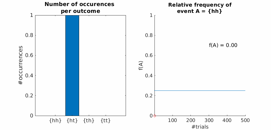
On the other hand, a low number of total observations does not give a good estimate of the true underlying probability of an event occurring. This is shown in the animation in Fig. 2, where we simulate the experiment of flipping two coins and we observe the number of times that each of the possible outcomes occurs. If we think about the probability of getting twice a head, we can already intuitively guess that it should be $1/4$. However, as shown in the right plot, we need about 500 trials to get an accurate estimation of this probability.

Thomas Bayes later offered a different interpretation of probability. This interpretation does not rely on the relative frequency of an event, but reflects a certain degree of belief that an event occurs. This probability is associated with a state-of-knowledge, influenced by a prior probability, which reflects the belief before an event actually takes place. As we will shall see, the Bayesian probability requires the calculation of prior probabilities; the principle of indifference and the classic definition of probability offer a source to calculate priopr probabilities that reflect ignorance (simplest, non-informative priors).

Example: Frequentist vs Bayesian perspective

Let us consider an extravagant example by calculating the probability of finding extraterrestrial life (aliens). From a frequentist perspective the probability of finding extraterrestrial life equals 0, because extraterrestrial life has not (yet) been observed. This provides us with a simple but limited answer to our question.

Now consider the Bayesian perspective. From scientific research we may conclude that extraterrestrial life is possible under the right circumstances. Combining this information with the immense number of planets, we could definitely argue for a non-zero probability of finding extraterrestrial life. This probability is regarded as the prior probability as it is determined without performing any observations. Even after performing many unsuccessful attempts at finding extraterrestrial life, there still is a (very small) probability of finding extraterrestrial life. The discrepancy in the probabilities is an example of the difference between the two definitions.

Probability axioms

From the definition of probability, three important probability axioms can be determined. Axioms are statements that are regarded as true and can therefore be used to prove other statements. The probability axioms are:

1. For any event $A$, it holds that $0\leq\Pr[A]\leq 1$.
2. It holds that $\Pr [\mathcal{S}]=1$.
3. For any countable collection of $M$ disjoint events it holds that $\Pr[A_1\cup A_2\cup \ldots \cup A_M] = \Pr[A_1] + \Pr[A_2] + \ldots + \Pr[A_M]$ .

Let us now discuss these axioms one by one. The first axiom states that a probability of an event is always between 0 and 1, where 0 means that there is no chance that the event will take place and 1 means that it will certainly happen; negative probabilities do not exist. Taking the frequentist definition of probability as a means to understand this, it is in fact not possible for an event to occur a negative number of times and therefore a negative probability cannot exist. Similarly, a probability larger than 1 would mean that a certain event would occur more often than all events together. Again this is not physically possible and therefore we are restricted to the probability bounds set by the first axiom.

The second axiom states that the probability of observing an outcome that is in the sample space $\mathcal{S}$ is always equal to 1. This axiom arises from the definition of the sample space. The sample space was defined previously as the set of all possible outcomes. Therefore we can conclude that an observation is always part of this set and thus the probability of observing an outcome that is part of the sample space equals 1.

The third axiom states that we may add the probabilities of separate events if we want to calculate the probability of the union of these events, under the constraint that the sets are disjoint to each other. Fig. 1 gives an intuitive explanation of why this holds. When the union of multiple disjoint events is calculated, there is no overlap (meaning no common outcomes) between these events. Therefore the total probability does not need to be compensated for overlap and we can simply add the probabilities of the separate events.

Consequences of the probability axioms

From the previous axioms, several consequences can be determined. These include:

1. It holds that $\Pr [\emptyset] = 0$.
2. It holds that $\Pr [A^C] = 1 - \Pr [A]$.
3. For any events $A$ and $B$ it holds that $\Pr[A\cup B] = \Pr[A] + \Pr[B] -\Pr[A\cap B]$.
4. If $A \subset B$ it holds that $\Pr[A] \leq \Pr[B]$.
5. For any event $A$ and event space $\{B_1, B_2, \ldots, B_m\}$ it holds that $\Pr[A] = \sum_{i=1}^{m}\Pr[A\cap B_i] = \sum_{i=1}^{m}\Pr[AB_i]$.

In 5., $\Pr[AB_i]$ indicates the probability of both events $A$ and $B_i$ occurring, that is the intersection. This also often indicated as $\Pr[A, B_i]$. So $\Pr[A \cap B_i] = \Pr[AB_i] = \Pr[A, B_i]$

The first consequence is rather straightforward. The probability of observing an outcome that is in the null event equals 0, because it reflects the chance that we observe nothing. This is not the case, since our observations are inevitably in the sample space.

The second consequence can be understood again through Fig. 1, where the definition of the complement plays an important role. The complement of an event $A$ includes all outcomes in the sample space except for all outcomes of event $A$. Since axiom 2 indicates that the probability of observing any outcome equals 1, the sets $A$ and $A^C$ together make up the entire sample space and therefore their probabilities should add up to one.

Consequence 3 is a generalization of axiom 3 and holds for all events, so not only for disjoint events. The axiom can be understood by analyzing Fig. 1. The union of two overlapping events can be written as their sum whilst compensating for the overlapping set of outcomes, denoted by the intersection of events. Therefore, the probability of the union of events $A$ and $B$ can be written as the sum of the individual probabilities minus the probability of the overlapping event. Axiom 3 is a special case of this axiom, where two events are disjoint and therefore the intersection between the two events equals 0.

The fourth consequence specifies that the probability of an event $A$ is smaller or equal to the probability of an event $B$ when $A$ is a subset of $B$. This is an immediate consequence of the definition of a subset, where the event $A$ contains a part of the outcomes of event $B$. Equality only occurs if the sets are equal.

The last consequence can be explained with the help of Fig. 3. The event $A$ can be split into multiple subsets, each in a separate region of the event space, denoted by the intersection between event $A$ and the subset $B_i$. Adding all different segments of $A$ gives the full event $A$, because the event space always covers the entire sample space and must therefore include the entire set of $A$.

Calculating probabilities

If we have enough information on an experiment and its associated sample space, we can calculate the probability of an event by using the probability axioms.

Example

Let us take look again at the experiment of rolling a dice twice and the event of obtaining both times head, i.e., $A=\{hh\}$. From the simulation in Fig. 2, we already know that the probability of this event should be 0.25. How can we reach the same conclusion without having to repeat the experiment hundreds of times? First, we gather the information we have on the experiment. We know that the sample space is given by $\mathcal{S} = \{ hh, ht, th, tt\}$. We also know the all the events in the sample space are disjoint and have equal probability. Thus, we can use the axiom of probability to write

\begin{eqnarray*} 1 &= &\Pr[ \mathcal{S} ] \newline &= &\Pr[\{ hh \}, \{ ht \}, \{ th \}, \{ tt \}] \newline &= &\Pr[\{ hh \}] + \Pr[\{ ht \}]+ \Pr[\{ th \}] + \Pr[\{ tt \}] \newline &= &4 \Pr[A], \end{eqnarray*}

from which can conclude that

\begin{equation*} \Pr[A] = \frac{1}{4} = 0.25. \end{equation*}

Conditional probability

Conditional probabilities describe our knowledge about an event, given the knowledge that another event has happened. As an intuitive example we could compare two situations. Suppose it is sunny outside and we want to know the probability that it starts raining. This probability is relatively low, whereas this probability would be a lot higher if it were cloudy. From this example, we may conclude that our knowledge of the weather at this moment, influences our prediction of raining in the near future.

A priori and a posteriori probability

The circumstances under which we would like to know the probability can be regarded as the observations of data. These observations provide us with insights about the circumstances and allow us to make a better estimate of the probability. The probability of an event $A$ occurring without having made any observations is called the a priori probability (prior = before) and is denoted by $\Pr[A]$. The a posteriori probability (post = after) is the new probability after having obtained more information about the situation. This probability is denoted as $\Pr[A|B]$, which is read as “probability $A$ given $B$”. In the previous example, $A$ could be regarded as the probability of raining in the near future and $B$ as the current weather.

This conditional probability $\Pr[A|B]$ can be calculated as \begin{equation} \Pr[A|B] = \frac{\Pr[AB]}{\Pr[B]}, \end{equation} where $\Pr[AB]$ is the probability of both events $A$ and $B$ occurring, which is equal to the probability of the intersection $\Pr[A\cap B]$. This equation scales the probability of observing an outcome in the intersection of $A$ and $B$ by the probability of $B$. From the visual notation of Fig. 1, this can be seen as the ‘area’ of the event $A\cap B$ normalized by the ‘area’ of $B$.

Properties of conditional probability

From the definition of this conditional probability, three properties can be deduced:

1. It holds that $\Pr[A|B] \geq 0$.
2. It holds that $\Pr[B|B] = 1$.
3. For a set of disjoint events $A = \{ A_1, A_2, \ldots, A_M\}$ it holds that $\Pr[A|B] = \Pr[A_1|B] + \Pr[A_2|B] + \ldots + \Pr[A_M|B]$.

Example: Frequentist vs Bayesian perspective

Let us consider again the experiment of flipping a coin twice, but this time we would like to calculate the probability of flipping two heads if we obtain a head in the first toss. Let $A_2$ be the event that you observe two heads, and $A_1$ be the event that you observe a head in the first toss. Using Eq. (4), we can write

\begin{equation*} \Pr[A_2|A_1] = \frac{\Pr[A_1 A_2]}{\Pr[A_1]}, \end{equation*}

To calculate $\Pr[A_1 A_2]$, we can observe that the event space of the intersection $A_1 \cap A_2 = \{hh\}$, that is the only outcome for which $A_1$ and $A_2$ both occurr, while the event space of $A_1$ is $A_1= \{hh, ht\}$. Thus, we can write

\begin{equation*} \Pr[A_1 A_2] = 0.25 \end{equation*}

\begin{equation*} \Pr[A_1] = 0.5 \end{equation*}

\begin{equation*} \Pr[A_2|A_1] = \frac{\Pr[A_1 A_2]}{\Pr[A_1]} = \frac{0.25}{0.5} = 0.5 \end{equation*}

Not surprisingly, the posterior probability of observing two heads ($\Pr[A_2|A_1]$) is different than its prior probability ($\Pr[A_2]$) due to the observation of an event that influences the final outcome.

Law of total probability

Similarly to the fifth consequence of the axioms of probability, a new expression can be determined using conditional probabilities. This is called the law of total probability and states that for an event space $\{ B_1, B_2, \ldots, B_M \}$ with $\Pr[B_i] > 0$ for all $i$, it holds that \begin{equation} \Pr[A] = \sum_{i=1}^{M}\Pr[A|B_i]\Pr[B_i]. \end{equation} This law inevitably follows from substituting the definition of the conditional probability as $\Pr[AB_i] = \Pr[A|B_i]\Pr[B_i]$ in the fifth consequence of the probability axioms.

Bayes’ theorem

One of the most important rules in probability theory is Bayes’ rule, which is obtained from the definition of the conditional probability. This conditional probability can be rewritten as \begin{equation} \Pr[A|B]\Pr[B] = \Pr[AB] = \Pr[BA] = \Pr[B|A]\Pr[A]. \end{equation} Equality of the middle two terms is obtained because these terms represent the same probability. Rewriting the leftmost and rightmost expression gives Bayes’ rule including the nomenclature of the separate terms as \begin{equation} \underbrace{\Pr[B|A]}_\text{posterior} = \frac{\overbrace{\Pr[A|B]}^\text{likelihood}\overbrace{\Pr[B]}^\text{prior}}{\underbrace{\Pr[A]}_\text{evidence}}. \end{equation}

Why is this particular notation so useful? The answer requires you to think in a certain context. Think of a context where an observation of an event $A$ is related to a (non-observable) underlying event $B$. An example of this context is where $A$ resembles the observed data and $B$ the model parameters creating this data. In the signal processing field we would like to obtain the model parameters to draw conclusions about the underlying process (for example in medical diagnostics). We would like to estimate these parameters after observing some data. Therefore we are interested in the probability $\Pr[B|A]$. However, we cannot determine this immediately and therefore we need Bayes’ rule. The initial (prior) probability of the model parameters is denoted by $\Pr[B]$ and is determined as an initial guess in terms of probability for the model parameters of the underlying process without having seen the data. The term $\Pr[A|B]$ represents the likelihood of the observed data under the assumed model parameters. Both of these terms can be calculated relatively easily. The last term $\Pr[A]$ represents the evidence, which is the probability of observing some data. This last term is usually more difficult to calculate and is therefore usually calculated by using the law of total probability.

Bayes’ theorem originates from a thought experiment, in which Bayes imagines to be sitting with his back at a perfectly flat, square table and he asks his assistant to throw a ball onto the table. The ball can land anywhere on the table, but Bayes wanted to guess where the ball was without looking at it. Then, he would ask the assistant to throw another ball on the table, and asked him whether the second ball fell to the left, right, up or down compared to the first one; he would note this down. Then, he would repeat this a number of times, and by doing so he could keep updating his belief on where the first ball was. Although he could never be completely certain, with each piece of evidence, he would a more accurate answer on the position of the first ball. Bayes’ theorem was in fact never meant as a static formula to be used once and put aside, but rather as a tool to keep updating our estimate as our knowledge about the experiment grows.

For a better undestanding of Bayes’ rule, you may take a look at the video and example below and try to solve the following exercise.