Introduction
Estimation theory is ubiquitous in our daily life and plays a fundamental role in many applications. The main objective of estimation theory is to infer the value of a parameter $\theta$. from some observations, which are represented by a vector $\mathbf{x}$ . These observations are random variables whose PDF depends on the unknown parameter. Thus, we denote the PDF as $p(\mathbf{x}; \theta)$ to emphasize its dependency on the parameter $\theta$.
Example:
Suppose we want to estimate a DC voltage $A$ which is embedded in noise. Our observation can be modeled as \begin{equation} x[n] = A + w[n], \end{equation} where $A$ is the unknown DC level, and w[n] is independent and identically distributed Gaussian noise with zero mean and known variance $\sigma^2$. The parametrized PDF of our observation is then \begin{equation} p(\mathbf{x};A) = \frac{1}{(2\pi\sigma^2)^{\frac{N}{2}}} \exp \left[-\frac{1}{2\sigma^2}\sum_{0}^{N-1}(x[n]-A)^2\right]. \end{equation}
An estimator is now a function $g(\mathbf{x})$ that maps from the observations $\mathbf{x}$ to an estimate $\hat\theta$ of the unknown parameter, i.e.,
\begin{equation}
\hat{\theta} = g(\mathbf{x}).
\end{equation}
Note that different estimators can be defined. For the previous example, we can define, for example, the following three estimators:
\begin{align}
\hat{A} &= \frac{1}{N} \sum_{n=0}^{N-1} x[n], \\\
\check{A} &= x[0], \\\
\tilde{A} &= \frac{1}{N-2}\left( 2x[0]+\sum_{n=1}^{N-2}x[n]+2x[N-1]\right).
\end{align}
The first estimator is the sample mean of the observation. The second estimator considers only the first observation, and the third estimator puts a higher weight on the first and the last observation. At this point, the question arises as to which of the estimators is the best. Furthermore, is there a better estimator? To answer these questions, we need first to define what we mean by best.
Since the observations $\mathbf{x}$ is a random vector, the estimate $\hat\theta$ is also a random variable. Thus, we need to evaluate an estimator by its statistic. First of all, it is desirable that an estimator produced the true parameter on average, i.e., \begin{equation} \mathbb{E}\left[\hat\theta\right] = \theta \end{equation} for all $\theta$.
An estimator with this property is said to be unbiased. Estimators for which the expected value approaches the true value as the sample size increases are called consistent estimators. All three presented estimators possess this property. Although unbiasedness is a preferred property, it does not help us answer which presented estimator is better. A more suitable criterion for the performance evaluation of an estimator is the variance of the estimate. The variance of a random variable reflects its variability. Thus, an estimator whose variance is small is desirable.
Returning to the three estimators. The individual variances of the estimates are:
\begin{align}
\mathrm{Var}\left[\hat{A}\right] &= \frac{\sigma^2}{N},\\\
\mathrm{Var}\left[\check{A}\right] &= \sigma^2,\\\
\mathrm{Var}\left[\tilde{A}\right] &= \frac{(N+6)}{(N+2)^2}\sigma^2.
\end{align}
When comparing the different variances, we see that the first estimator has the lowest variance. When compared to the second estimator, we see that the variance is $N$-times smaller due to the noise averaging effect of the estimator. The variance of the last estimator converges to the variance of the first estimator as the sample size increases.
So far, we have seen that we can formulate different estimators, and we can compare their performance by means of their variance. It is logical now to ask if other estimators can have a lower variance or even a variance equal to zero. In this part of the lecture, we will answer this question and show that there exists a lower bound on the variance for unbiased estimators. Moreover, the bound provides an equality constraint which allows us to find an estimator with a variance equivalent to this bound. Such estimators are referred to as efficient estimators. In fact, the sample mean $\hat{A}$ in the above example is such an estimator. In general, efficient estimators only exist for special cases. Thus, we are interested in finding an estimator which has the lowest variance of all unbiased estimators. An estimator whose variance is lower then the variance of all other unbiased estimators for all values of $\theta$ is termed minimum variance unbiased estimator, or short MVUE. It should be noted that such an estimator must not necessarily exist and if it exits, it must not necessarily be unique.
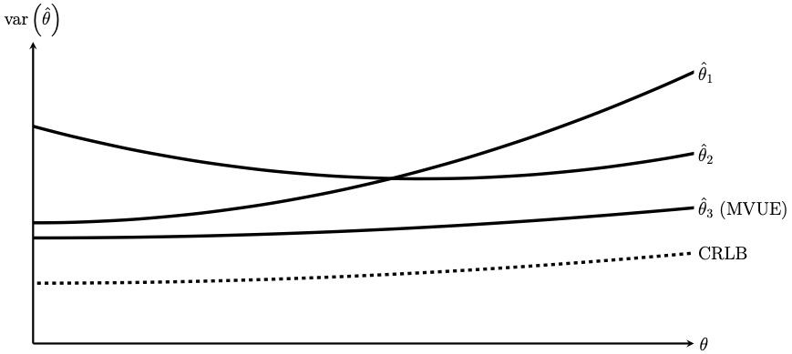
An example of the different behavior of the variance is provided in the figure below. As shown, the variance can depend on the unknown parameter $\theta$. In particular, the variances of one estimator may be locally be better than the variance of another estimator. In the example below, $\hat\theta_1$ and $\hat\theta_2$ are performing for a specific range better than the other one. However, $\hat\theta_3$ is performing better than the other two for the entire range. Thus, $\hat\theta_3$ is the MVUE.
Outline
The topics covered in this part are
- The Cramer-Rao Lower Bound: Just as the data is stochastic, so are the parameter estimations. When the noise properties are known, the lowest possible variance for the parameter estimations can be calculated for unbiased estimators.
- Maximum Likelihood Estimator: The stochastic nature of the data due to the noise is modeled in terms of the probability density function of the noise. The parameter value that maximizes the probability of observing the data at hand is the maximum likelihood estimate.
- Minimum Variance Unbiased Estimator and Best Linear Unbiased Estimator: The minimum variance unbiased estimator can be found for linear problems with Gaussian noise.
- The Cramer-Rao Lower Bound: Just as the data is stochastic, so are the parameter estimations. When the noise properties are known, the lowest possible variance for the parameter estimations can be calculated for unbiased estimators.
- Maximum Likelihood Estimator: The stochastic nature of the data due to the noise is be modeled in terms of the probability density function of the noise. The parameter value that maximizes the probability of observing the data at hand is the maximum likelihood estimate.
- Maximum Likelihood Estimator: The stochastic nature of the data due to the noise is modeled in terms of the probability density function of the noise. The parameter value that maximizes the probability of observing the data at hand is the maximum likelihood estimate.